The Main Toolkit file contains a user-entered transportation network consisting of a series of nodes (intersections) and directional links (road segments). Additional information is required, such as traffic link volumes, roadway capacity, tolls, etc., though many inputs are optional and may be used for more detailed analysis. The user then enters into the Main Toolkit File the ways in which the transportation network will change then runs the Travel Demand Model (composed of the Trip Table Estimator and Network Flow Estimator). The Main Toolkit File will read in the Travel Demand Model's outputs and report how travel patterns and traffic impacts change in the base case and alternative scenarios.
Once the analyst has specified the transportation network, alternative network(s), current traffic volumes and parameters in the Main Toolkit File, the analyst may run the Trip Table Estimator. This component estimates current traffic flows between all origins and destinations for each time of day. It should be noted that every node is a potential origin and potential destination for all other nodes.
For more information, see Section 9.0 of the Toolkit User's Guide.
After trip tables have been established, the Network Flow Estimator may be run from the Main Toolkit File. This will assign traffic volumes by link, time of day, user class, and mode for a given scenario (base-case, alternative 1, 2 or 3) and year (initial or design). Total scenario traveler welfare estimates are also generated using the Network Flow Estimator. The Network Flow Estimator is typically run multiple times to estimate traffic impacts in each scenario for both the initial and design years.
For more information, see Section 9.0 of the Toolkit User's Guide.
There are two ways to enter data into PET, through the Main Toolkit File or through the Toolkit Upload File. Entering data into PET through the Main Toolkit File may be conducted by entering network, parameter, or other input information. This works fine for small edits and developing new scenarios, but can be laborious if a significant amount of input data is required (for example, developing a new network from scratch). The Main Toolkit File contains numerous formulas and there is a small processing delay each time a new value is entered.
In order to address this issue and provide a convenient location for all inputs, the analyst may opt to use the Toolkit Upload File. This file contains data entry locations for the vast majority of inputs, which may then be quickly uploaded to the Main Toolkit File once all inputs have been entered.
For more information, see Section 2.3 of the Toolkit User's Guide.
Most components of the Project Evaluation Toolkit are designed as an alternative analysis tool which may be used to identify desirable project scenario alternatives. The budget allocation module may be used to identify a preferred mix of potential projects in order to achieve the maximum benefits. Analysts may specify budget limits and equity considerations, such as ensuring that various regions have minimum expenditure levels. Moreover, the budget allocation module requires the analyst to specify a pre-determined level of required investment for every candidate project, under the assumption that one project's costs will not impact another project's cost. In this regard, the budget allocation decision making process will choose mix of projects that will deliver the maximum benefits, within the limits of budget and other constraints.
For more information, see Section 12.0 of the Toolkit Users Guide.
PET’s multi-objective decision-making tool (MODMT) enables engineers,
planners and others to select one or more optimal projects or scenarios from
among competing alternatives subject to multiple criteria that are not all
monetized or reduced to a single type of unit (e.g., not all are resolved in
minutes saved or dollars saved). The MODMT uses a Data Envelopment Analysis,
a methodology that uses an “efficiency” value to rank different scenarios.
Scenarios whose efficiency is less than one are clearly dominated by other
scenarios, and are not recommended; the scenarios with an efficiency greater
than or equal to one are candidates which are potentially optimal, depending
on one’s relative valuation of the different criteria. The magnitude of the
efficiency value reflects the degree to which these scenarios are dominated
(or not) by the others and this method is not sensitive to the units used
for each criterion.
For more information, see Section 13.0 of the Toolkit Users Guide.
PET uses a travel demand forecasting module to estimate how traffic patterns change as a result of changes travel demand over time, and changes in the overall transportation network as compared to current conditions. The module is designed to strive to closely mimic large, full-size network demand estimation results across different roadway facilities, times of day, and changed network conditions.
PET's travel demand model uses five major steps to assign traffic flows among transportation modes, across time of day (TOD) periods, and over the network. These produce a base trip table estimate, elastic trip table estimates for each scenario, mode split and time of day estimates, and link-based traffic assignments (for each traveler class modeled). Once the traffic assignment process is complete, the model checks for convergence (using traffic flow stability as described later) and loops back to the elastic trip table estimation process if convergence has not been reached, as shown in the above Figure.

PET's Travel Demand Modeling Process
The first step estimates an origin-destination (O-D) trip table based on link traffic counts (AADT
values). This process assumes that route choices rely on stochastic user
equilibrium. Future-year travel demands between each O-D pair for the base-case (no-build) option are based on a user-assumed travel growth rates.
The second step uses an elastic demand function to estimate cost-dependent O-D trip rates for all other scenarios, by pivoting off of the base-case trip rates using an assumed demand elasticity for each time of day (-0.69 default for all periods).
The third step, mode split, uses an incremental multinomial logit (MNL) model to distribute the O-D trips (as developed in the second step) into different transportation modes, such as drive-alone, shared-ride modes, and transit.
The fourth step also uses an incremental MNL model to produce trip tables by time of day for each transportation mode.
The fifth step assigns these various trip tables (by vehicle type, traveler class, travel mode, and time of day) to the abstracted/coded network under the user-equilibrium principle.
The last four steps form a supply-demand interaction loop and are conducted iteratively, using a feedback mechanism. This ensures that flows and costs are in equilibrium, between different times of day, across transportation modes, and across network routes. The feedback process iterates until the consistency between traffic flows and travel costs are reached.
For more information, see Section 9.0 of the PET User's Guide.
How does PET estimate impacts?
PET assesses six major impacts:
- Traveler Welfare (consisting of operating costs and changes in travel time)
- Travel Time Reliability (based on the valuation of travel time variance)
- Crash Counts (by severity)
- Emissions Quantities (14 species)
- Tolling Revenues
- Fuel Use
All traveler welfare impacts are evaluated at the origin-destination level while all other impacts are evaluated at the individual link level.
Traveler Welfare
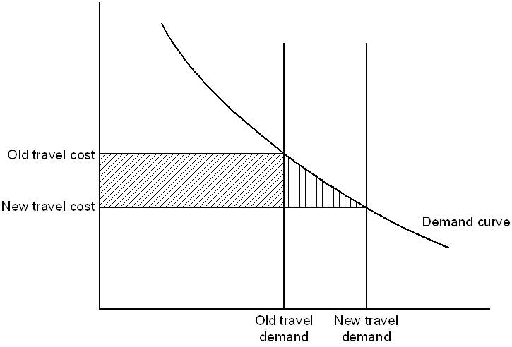
Traveler welfare is estimated as a function of monetized travel time changes and operating costs, while accounting for benefits to new travelers between each origin-destination pair due to reduced costs, or disbenefits to prior travelers who no longer travel between the origin-destination pair due to increased costs.
Traveler welfare (sometimes referred to as consumer surplus) changes are approximated using the rule-of-half (RoH) method. This assumes linear demand curves between O-D pairs, and is quite reasonable in the presence of non-linear response for relatively moderate changes in network performance. A graphical illustration of this estimation process between a single origin-destination pair, is shown in the figure below, with benefits consisting of the shaded components.
For more information on Traveler Welfare impact estimation, see Section
10.1 of the PET
User's Guide.
Travel Time Reliability
The Project Evaluation Toolkit anticipates uncertainty in travel times, so that such values may be summed over connecting links, along with travel times for route choices. Such uncertainty is estimated as the convex relationship between freeway volume-capacity ratios and travel time variances using freeway traffic data. This estimated relationship is graphically depicted in the figure below.
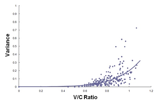
PET multiplies travel time unreliability by each user's value of reliability (VOR) and sums over all links to determine the total system reliability costs. The default value of VOR (in terms of hours of standard deviation in travel time) is assumed to equal each traveler type's respective value of travel time (VOTT).
For more information on Traveler Welfare impact estimation, see Section
10.2 of the PET
User's Guide.
Crash Counts
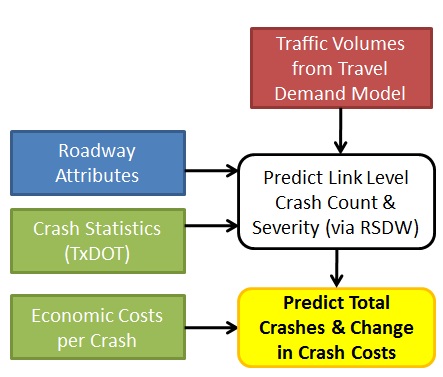
Crashes are predicted using safety performance functions (SPFs) derived from the Road Safety Design Workbook. These SPFs allow users to pivot off existing crash rates and crash counts to estimate future numbers of fatal, injurious (F+I) and property-damage-only (PDO) crashes on each link in the system. Key factors are link functional classification, AADT, and number of lanes. Segment (link) crashes are estimated for all coded roadway types, and intersection crashes are estimated for arterials and rural roads. Crash modification factors (CMFs) may be applied to individual links or intersections in order to obtain more accurate crash predictions.
The Project Evaluation Toolkit estimates crash severity based on TxDOT motor vehicle crash statistics. A set of fixed shares of crash severity outcomes (proportions of fatal, incapacitating injury, non-incapacitating injury, possible injury and property damage only) was assumed for all rural crashes and another set of fixed shares of crash severity outcomes for all urban crashes. This process is shown in the figure below.
For more information on Crash Count estimation, see Section 10.3 of the PET
User's Guide.
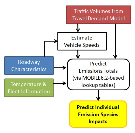
Emissions Quantities
Vehicle emission quantities are predicted using lookup tables generated by the EPA's
new MOVES model. These lookup tables estimate individual emission outputs in grams per mile for
14 species, with five representing mobile-source air toxics, or MSATs. Emissions rates depend on facility type (freeway, arterial, local road, or ramp); vehicle speed (14 speed categories—from 2.5 mph and slower to 65 mph and faster); temperature range (four temperature ranges, with 30 degrees at the low end and 105 at the high end); year of analysis (based on analysis year closest to 2010, 2015, 2020, or 2025, and impacting vehicle ages [and thus rates]); vehicle type (28 types); and vehicle age (6 age categories in 5-year increments). PET estimates link-level emissions based on the total number of light (8500 lbs. and under) and heavy vehicles on a link as well as the link's classification and speed estimates. This process is shown in the figure below.
For more information on Emissions Quantities estimation, see Section 10.4 of the PET
User's Guide.
Tolling Revenues
Tolling revenues are assessed at the individual link level, based on the number of and type of vehicles traveling on that link for each time of day, and the corresponding toll price. Toll revenues are also not included in the summary measures (such as Net Present Value and Benefit/Cost Ratios) because their direct impact should be neutralized by the transfer of traveler monies to tolling agencies. In other words, this cost to travelers is an equal dollar benefit to road authorities, excluding the cost of toll collection and overhead. This being noted, a financing module is also included so that agencies can determine if the tolling revenues will be sufficient to cover the cost of project construction and annual maintenance and operations.
Fuel Use
PET estimates individual traveler fuel consumption as a function of vehicle speeds and average fleet fuel economy. Total fuel use is the sum of estimated fuel rate consumed on each link. Fuel use is also excluded from the summary measures as an independent impact, since its impacts are already accounted for in vehicle operating costs, which is a component of the Traveler Welfare estimation.
For more information on Fuel Use estimation, see Section 10.5 of the PET
User's Guide.
I've run PET. Which alternative should I choose?
PET provides analysts with the ability to anticipate project outcomes. The most important measures that users will likely focus on are the reported Net Present Value (NPV), Benefit Cost Ratio (B/C Ratio), Payback Period (PP), and Internal Rate of Return (IRR). Transportation planners and decision makers will typically select their preferred alternative based on one of these measures.
This being noted, users should be aware that there are other measures that they may wish to account for that are reported by PET but not included in the summary measures. These include emissions costs, non-market or "soft" crash costs (such as pain, suffering and the value of life), fuel consumption (included as a component of traveler welfare) and tolling revenues. Optionally, users may assign values to emissions or the value of life to move these components into the summary measure evaluations. Conversely, components such as travel time reliability may be omitted from the summary measures by setting values of reliability to zero. Impacts not included in the summary measures may still be incorporated into the final selection process by using weighted-ranking schemes or other selection methods. Also, tolling revenue impacts may be assessed separately using the project financing module. The various cost and benefit component measures are shown in the figure below.

How are impacts assessed over time?