UTCHEM BIODEGRADATION MODEL
DESCRIPTION AND CAPABILITIES
Phillip C. deBlanc, Daene C. McKinney, Gerald E. Speitel,
Jr.
Center for Research in Water Resources
Mojdeh Delshad, Gary A. Pope, Kamy Sepehrnoori
Center for Petroleum and Geosystems Engineering
University of Texas at Austin
April 5, 1996
1.0 INTRODUCTION
UTCHEM is a multi-phase, multi-component, three-dimensional, numerical model
that simulates the fate and transport of both dissolved and non-aqueous
phase organic contaminants in porous media. The model can be used to simulate
spills of either lighter-than-water NAPLs (LNAPLs) or denser-than-water
NAPLs (DNAPLs). The NAPL phase can contain up to five organic constituents.
The transfer of organic contaminants from the NAPL to the aqueous phase
is described through either equilibrium partitioning or a linear driving
force non-equilibrium mass transfer model. Adsorption of organic constituents
is modeled through equilibrium partitioning. An arbitrary number of injection
and pumping wells can be specified so that bioremediation schemes can be
modeled and bioremediation designs can be optimized. The previous version
of the UTCHEM model is described in detail by Delshad et al. (1996).
Advanced biodegradation capabilities have recently been incorporated into
UTCHEM. The biodegradation option allows an entirely new class of problems
to be simulated with UTCHEM, such as surfactant remediation followed by
biodegradation of the residual surfactant and contaminant. This document
describes the biodegradation model capabilities, presents and explains the
biodegradation equations, and provides examples of UTCHEM biodegradation
simulations.
2.0 CURRENT MODEL CAPABILITIES
UTCHEM simulates the biodegradation of chemical compounds that can serve
as substrates (carbon and/or energy sources) for microorganisms. The model
simulates the destruction of substrates, the consumption of electron acceptors
(e.g. oxygen, nitrate, etc.), and the growth of biomass. Substrates can
be biodegraded by free-floating microorganisms in the aqueous phase or by
attached biomass present as microcolonies in the manner of Molz et al.
(1986). Multiple substrates, electron acceptors and biological species are
accommodated by the model. Important assumptions for the biodegradation
model are:
- Biodegradation reactions occur only in the aqueous phase.
- Microcolonies are fully penetrated; i.e., there is no internal resistance
to mass transport within the attached biomass.
- Biomass is initially uniformly distributed throughout the porous medium.
- Biomass is prevented from decaying below a lower limit by metabolism
of naturally occurring organic matter unless cometabolic reactions act to
reduce the active biomass concentrations below natural levels.
- The area available for transport of organic constituents into attached
biomass is directly proportional to the quantity of biomass present.
The biodegradation model includes the following features:
- Monod, first-order, or instantaneous biodegradation kinetics.
- Formation of biodegradation by-products.
- External mass transfer resistances to microcolonies (mass transfer resistances
can be removed by the user if desired).
- Inhibition of biodegradation by electron acceptors and substrates toxic
to microorganisms.
- Nutrient limitations to biodegradation reactions.
- First-order abiotic decay reactions.
- Enzyme competition between multiple substrates.
- Modeling of cometabolism with reducing power limitations and finite
transformation capacities using the model of Chang and Alvarez-Cohen (1995).
- Biodegradation reactions in both the vadose zone and under fully water
saturated conditions.
Examples of how these features are used in biodegradation modeling are provided
below.
Example 1 - Biodegradation of benzene, toluene, ethylbenzene, and
xylene (BTEX) from a gasoline spill
UTCHEM can simulate the biodegradation of each BTEX compound individually
or as a pseudo-component using average biodegradation kinetic parameters.
The model simulates the aerobic destruction of the BTEX, the development
of an oxygen-deficient zone downgradient of the spill, and the dissolution
of the BTEX compounds from any free-phase gasoline present. If nitrate is
assumed to be present in the water, then the model can use electron acceptor
inhibition functions to "switch off" aerobic biodegradation and
"switch on" anaerobic biodegradation of toluene, ethylbenzene
and xylene where oxygen concentrations are sufficiently low. Low concentrations
of nutrients, such as nitrogen and phosphorous, also limit biodegradation
reactions through nutrient Monod terms.
Example 2 - Aerobic biodegradation of trichloroethene (TCE)
TCE can be biodegraded with oxygen as the electron acceptor by methanotrophs
that use methane as the primary carbon and energy source (McCarty, 1993).
UTCHEM can model the mineralization of TCE under aerobic conditions. Methane
competes with TCE for the enzyme that degrades the two compounds, resulting
in lower rates of TCE biodegradation that might otherwise be anticipated.
UTCHEM includes enzyme competition kinetics to take this competitive inhibition
of TCE into account. Where methane is not present to act as a growth substrate,
the biomass is deactivated by cometabolic reactions which "drain"
reducing power from the microorganisms. The model also simulates the reduction
in active biomass caused by highly reactive reaction intermediates through
finite transformation capacities.
Example 3 - Anaerobic biodegradation of TCE by cometabolism
TCE can also be biodegraded anaerobically under methanogenic conditions
to dichloroethene (DCE), which in turn can be biodegraded into vinyl chloride
(VC) (Vogel, 1993). The entire process can be simulated by UTCHEM. UTCHEM
can simulate the generation of DCE as a product of TCE biodegradation, and
the production of VC as a by-product of DCE biodegradation. Biodegradation
is repressed where oxygen is present through the electron acceptor inhibition
functions. Reduced biodegradation rates near the TCE source, where high
concentrations of TCE may be toxic to microorganisms, is modeled with a
substrate inhibition term.
Example 4 - Anaerobic biodegradation of 1,1,1-trichloroethane (1,1,1-TCA)
As a final example, the anaerobic conversion of 1,1,1-TCA to 1,1-dichloroethane
and then to chloroethane (CA) can be modeled by UTCHEM. CA can be converted
abiotically into ethanol and chloride through hydrolysis reactions (McCarty,
1993). TCA can also be transformed directly into 1,1-DCE and acetic acid
via abiotic reactions (McCarty, 1993). UTCHEM can simultaneously model both
the biological reactions that convert 1,1,1-TCA to CA, the abiotic transformation
of CA to ethanol and chloride, and the abiotic transformation of TCA to
DCE and acetic acid.
3.0 BIODEGRADATION EQUATIONS AND SOLUTION PROCEDURE
The biodegradation model equations describe the transport of substrate and
electron acceptor from the aqueous phase into attached biomass, the loss
of substrate and electron acceptor through biodegradation reactions, and
the resulting growth of the free-floating or attached biomass. The flow
and biodegradation system is solved through operator splitting, in which
the solution to the flow equations is used as the initial conditions for
the biodegradation reactions. This approach is convenient because modifications
can be made to the system of biodegradation equations without having to
reformulate the partial differential equations that describe advection and
dispersion.
The biodegradation equations comprise a system of ordinary differential
equations that must be solved at each grid block and each time step after
the advection and dispersion terms are calculated. Because the mass transfer
terms can make the system of equations stiff, the system is solved using
a Gear's method routine published by Kahaner et al. (1989). The characteristics
and numerical solution of this system of equations is discussed by de Blanc
et al. (1996).
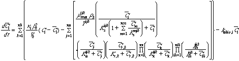
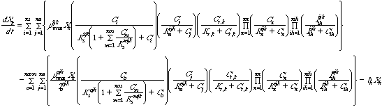
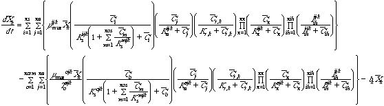
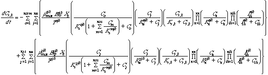
The complete system of equations is presented in Table 1. A key to the symbols
in these equations is included in Table 2.
Equation 1 describes the three mechanisms for loss of substrate in the aqueous
phase. The first expression describes diffusion of substrate across a stagnant
liquid into attached biomass. The second expression in Equation 1 describes
the biodegradation of substrate by unattached microorganisms in the bulk
liquid. The first Monod term in this expression accounts for substrate limitations
on the reaction rate and incorporates substrate competition. The second
Monod term accounts for reaction rate limitations by the electron acceptor.
The third Monod term accounts for reducing power limitations on the reaction
rate if cometabolism is causing a loss of reducing power in the biomass.
The first product of Monod terms limits the reaction rate because of the
concentration of any other compound needed for growth, such as nutrients
like nitrogen or phosphorous. The second product term limits the reaction
rate through inhibition. The inhibiting compound(s) can be another electron
acceptor, a toxic reaction by-product, or the substrate itself. As many
of these additional Monod terms as are needed can be specified in the model.
The third expression accounts for abiotic loss of the substrate through
first-order reactions.
One equation similar to Equation 1 is written for each substrate. One equation
similar to Equation 1 is also written for each chemical constituent that
appears in the biodegradation kinetic expression, including electron acceptors,
nutrients, and inhibiting compounds, but not including NADH. Finally, one
equation similar to Equation 1 is written for each product. The biodegradation
expression for product generation, electron acceptor use and nutrient use
are multiplied by a factor Eijk, which is the stoichiometric ratio
of the mass of the other compound lost (or generated) per mass of substrate
biodegraded.
Equation 2 is a mass balance equation written for a single microcolony in
the manner of Molz et al. (1986) This equation describes the diffusion
of substrate into the biomass and the biodegradation of the substrate within
the biomass. Substrate competition and inhibition are incorporated into
the biodegradation expression in the same manner as in the bulk liquid biodegradation
expression. Equations similar to these are written for product generation,
electron acceptor use, and nutrient use. One of these equations is required
for each substrate, electron acceptor, nutrient, and inhibiting compound.
Equations 3 and 4 describe the growth and decay of unattached and attached
biomass, respectively. If there is cometabolism, then the equations describe
the growth and loss of active biomass rather than total biomass.
The loss of biomass due to cometabolism is expressed through the transformation
capacity, Tc, which is the ratio (cometabolite biodegraded/biomass
consumed). The cometabolic model is based on the model of Chang and Alvarez-Cohen
(1995). The third expression in these equations describes the loss of biomass
through endogenous decay. One of each of these equations is written for
each biological species.
Equations 5 and 6 describe the consumption of reducing power (NADH) by cometabolic
reactions and the regeneration of reducing power by growth substrates. Inclusion
of a reducing power limitation for cometabolism is optional in the program.
One of each of these equations is required for each biological species that
cometabolizes a substrate.
The effect of the Monod and inhibition terms, and the mass transfer limitations
on the biodegradation kinetics is described in more detail by de Blanc et
al. (1995). This complex system of ordinary differential equations is
solved at each grid block and each time step by Gear's method using subroutine
SDRIV2 published by Kahaner et al.
4.0 MODEL TESTING AND VALIDATION
The biodegradation component of UTCHEM has been extensively tested to ensure
that correct solutions to the biodegradation equations are produced. The
testing consisted of batch biodegradation simulations, in which the solutions
to the equations provided by the model for simple systems were compared
to solutions calculated in spreadsheets.
Complete biodegradation solutions were also compared against literature
solutions to ensure that the simultaneous transport and biodegradation of
substrates and electron acceptors produced reasonable results. One-dimensional,
single-phase simulations have been compared to biodegradation model solutions
published by Molz et al. (1986). Substrate profiles generated by
the two models in one such comparison are shown in Figure 1. In this simulation,
a single substrate is biodegraded by attached biomass using oxygen as the
electron acceptor. The simulation results are very similar to the data of
Molz et al. (1986), indicating that the UTCHEM biodegradation model
is functioning properly. The model predictions are not exactly the same
because of slightly different assumptions about endogenous decay and slightly
different flow conditions.
5.0 EXAMPLE SIMULATIONS
The multi-phase flow and biodegradation capabilities of the model are demonstrated
through the simulation of hypothetical LNAPL and DNAPL spills. In these
simulations, the modeling domain consists of a confined aquifer that is
125 m long by 54 m wide by 6 m thick. The domain is simulated with 25 grid
blocks in the x direction, 11 grid blocks in the y direction, and 5 grid
blocks in the z direction. Groundwater is flowing from left to right with
an average velocity of 0.1 m/day. The spills are modeled by injecting the
NAPL into the center of grid block (5, 6, 1), which is approximately 22
meters from the left boundary in the center of the modeling grid. There
is no air phase in these simulations; the top boundary is a no-flow boundary.
LNAPL Simulation Example
Sequential use of electron acceptors and partitioning of multiple components
into the aqueous phase are illustrated with an example LNAPL simulation.
The LNAPL example simulates a leak of 1,000 gallons of crude oil containing
approximately 1% by volume of benzene and 6% by volume of toluene into a
shallow, confined aquifer. The leak is assumed to occur over a four-day
period.
Figure 2 shows the evolution of the oil lens in a vertical slice down the
center of the aquifer in the x-z plane. As seen in Figure 2, the oil moves
little once the oil lens is established. The oil lens gradually decreases
in size as the organic constituents dissolve into the flowing groundwater.
As the benzene and toluene partition out of the crude oil into the aqueous
phase, they become available to microorganisms as substrates. For simplicity,
a single population of microorganisms capable of biodegrading the benzene
and toluene is assumed to exist in the aquifer. This biological species
biodegrades both benzene and toluene aerobically and biodegrades toluene
anaerobically with nitrate as the electron acceptor. Biodegradation kinetic
parameters used for the simulation were obtained from Chen et al.
(1992).
Figure 3 compares the concentration of benzene in the aqueous phase at 500
days to the concentration of benzene that would exist if no biodegradation
reactions were occurring. The figure shows that significant biodegradation
of dissolved benzene has occurred. The toluene plume is also shown in Figure
3. Although toluene has a lower solubility than benzene, the maximum toluene
concentration in the dissolved phase is higher than the maximum concentration
of the benzene plume because its concentration in the crude oil is greater
than the benzene crude oil concentration. Toluene concentrations are nearly
as low as benzene concentrations at the fringes of the plume because toluene
is biodegraded both aerobically and anaerobically, where oxygen is exhausted,
but the benzene is not.
The concentrations of benzene, toluene, oxygen and nitrate at 500 days are
compared in Figure 4. Oxygen immediately downgradient of the spill is practically
exhausted. Nitrate is also nearly exhausted from the area immediately downgradient
of the spill because sufficient time has elapsed since oxygen depletion
to allow denitrification to occur. However, at the forward edge of the plume,
relatively high nitrate concentrations still exist in areas where oxygen
has been depleted, but not exhausted.
DNAPL Simulation Example
Different model capabilities are illustrated with a DNAPL simulation in
which TCE is biodegraded through cometabolism. In this simulation, 7.5 gallons
of TCE is spilled in a single day. The cometabolic process is illustrated
by injecting water containing methane through five injection wells located
approximately 24 meters downgradient of the spill. The water contains 20
mg/L methane and 8 mg/L oxygen. The water injection rate is 1.4 m3 per day
per well.
A population of methanotrophic microorganisms capable of biodegrading TCE
aerobically through cometabolism is assumed to exist in the aquifer. The
methanotrophs use methane as the primary substrate and oxygen as the electron
acceptor. TCE biodegradation is assumed to reduce the active biomass and
consume reducing power of the methanotrophs, so that TCE biodegradation
both reduces the active biomass concentration and reduces the active biomass's
biodegradation effectiveness. Once biomass has become deactivated, it does
not become active again. Biodegradation rate parameters were obtained from
Chang and Alvarez-Cohen (1995).
The effect of the methane injection wells is illustrated in Figure 5, where
concentrations of TCE, a hypothetical TCE tracer, oxygen and methane are
shown at 170 days. The TCE tracer is simply TCE that is not allowed to biodegrade
in the model so that the effects of biodegradation can be seen. Concentration
contours of the different constituents are shown in the top 1.2-m layer
of the aquifer. Oxygen is depleted downgradient of the plume, but only a
small fraction of the oxygen is consumed upgradient of the methane injection
wells. Most of the oxygen upgradient of the wells remains because the high
TCE concentrations deactivate the biomass and consume reducing power, preventing
the TCE from biodegrading and further depleting the oxygen.
Even with a small TCE spill, TCE concentrations in the aquifer are so high
that most biomass immediately downgradient of the spill is deactivated.
Significant TCE biodegradation occurs only where appreciable methane is
present to regenerate the microorganism's reducing power and where TCE concentrations
are low. These effects can be seen in Figure 5. The high concentration contours
of the TCE and TCE tracer are nearly the same, but biodegradation of the
TCE causes a slight retardation in the progress of the TCE plume at low
concentrations.
5.0 FUTURE MODEL ENHANCEMENTS
The UTCHEM biodegradation model is continually being refined. The following
capabilities are planned for inclusion in the model prior to its completion:
· Biomass transport;
· Biomass growth limitations to prevent unbridled biomass growth;
· Effects of biomass growth on porosity and permeability;
· Incorporation of lag times to account for biomass acclimation.
6.0 REFERENCES
Chang, H. and L. Alvarez-Cohen, Model for the cometabolic biodegradation
of chlorinated organics, Environmental Science and Technology, 29(9):
2357-2367, 1995.
de Blanc, P., D. C. McKinney and G. E. Speitel, Jr., Modeling subsurface
biodegradation of non-aqueous liquids: a literature review, Technical
Report CRWR 257, University of Texas at Austin, February, 1995.
de Blanc, P. C., K. Sepehrnoori, G. E. Speitel Jr. and D. C. McKinney, Investigation
of numerical solution techniques for biodegradation equations in a groundwater
flow model, Proceedings of the XI International Conference on Computational
Methods in Water Resources, Cancun, Mexico, July 22-26, 1996 (in press).
Delshad, M., G. A. Pope and K. Sepehrnoori, A compositional simulator for
modeling surfactant enhanced aquifer remediation, In press, Journal of
Contaminant Hydrology, 1996.
Kahaner, David, C. Moler and S. Nash, Numerical Methods and Software,
Prentice Hall, Englewood Cliffs, NJ, 1989.
Molz, F. J., M. A. Widdowson and L. D. Benefield, Simulation of microbial
growth dynamics coupled to nutrient and oxygen transport in porous media,
Water Resources Research, 22(8): 1207-1216, August 1986.
McCarty, P. L. and L. Semprini, Ground-water treatment for chlorinated solvents,
In: Handbook of Bioremediation, (J. E. Mathews project officer),
Lewis Publishers, Boca Raton, FL, pp. 87-116, 1993.
Vogel, T. M., Natural bioremediation of chlorinated solvents, In: Handbook
of Bioremediation, (J. E. Mathews project officer), Lewis Publishers,
Boca Raton, FL, pp. 201-224, 1993.
TABLE 1
BIODEGRADATION EQUATIONS
Equation 1 Substrate loss in the bulk fluid:

Equation 2 Substrate loss in attached biomass:
Equation 3 Growth of unattached biomass:
Equation 4 Growth of attached biomass:
Equation 5 Reducing power (NADH) consumption and production in
unattached biomass:
Equation 6 Reducing power (NADH) consumption and production
in attached biomass:
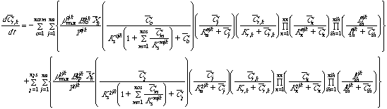
TABLE 2
KEY TO SYMBOLS IN BIODEGRADATION EQUATIONS
Letters:
b Endogenous decay coefficient (T-1)
Ci concentration of species i in bulk liquid (mass C/volume of aqueous
phase)
Ci concentration of species i within attached biomass (mass C/volume
of biomass)
Eijk electron acceptor use coefficient of electron acceptor j for
biodegradation of substrate i by bacterial species k (mass electron acceptor
consumed/mass substrate consumed)
Iaijk electron acceptor inhibition constant for biodegradation of
substrate i by bacterial species k using electron acceptor j (mass/volume
of phase)
Isijk substrate self-inhibition constant for biodegradation of substrate
i by bacterial species k using electron acceptor j (mass/volume of phase)
kabio first-order abiotic reaction coefficient
Kaijk Monod half-saturation constant for electron acceptor j under
j-based metabolism of substrate i by bacterial species k (mass A/volume
of phase)
Kr Monod half-saturation constant for NADH growth limitations (mass/volume
of phase)
Ksijk Monod half-saturation constant for substrate i under j-based
metabolism by bacterial species k (mass /volume of phase)
mk mass of a single bacterial colony (mass/colony)
t time (T)
Tc transformation capacity (mass of biomass deactiveated/mass of
cometabolite biodegraded)
Vk volume of a single bacterial colony (volume/colony)
Xk concentration of attached biomass k (mass/volume of aqueous phase)
Xk concentration of free-floating biomass k (mass/volume of aqueous phase)
Yijk yield coefficient for component i under j-based metabolism
by bacterial species k (dimensionless; mass of biomass produced/mass of
substrate utilized)
Greek Letters:
i mass transfer coefficient of species i (L/T)
[[beta]] surface area of a single bacterial colony available for
mass transfer (L2/colony)
uijkmax Monod maximum growth rate for component i under j-based metabolism
by bacterial species k (T-1)
[[rho]]k biomass density (active biomass/volume of biomass)
TABLE 2
KEY TO SYMBOLS IN BIODEGRADATION EQUATIONS
Subscripts:
c cometabolite
i substrate
ih inhibiting compound
j electron acceptor
k biological species
m competing substrate
n nutrient
na number of electron acceptors
nb number of biological species
ncom number of cometabolites
ncs number of competing substrates
nih number of inhibiting compounds
nn number of nutrients
ns number of substrates
r reducing power (NADH)
Superscripts such as ijk refer to metabolic combinations of substrate, electron
acceptor and biological species. 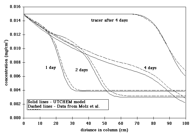 Figure 1. Comparison
of substrate profiles simulated by UTCHEM to column profiles simulated by
the model of Molz et al. (1986) in a laboratory column.
Figure 1. Comparison
of substrate profiles simulated by UTCHEM to column profiles simulated by
the model of Molz et al. (1986) in a laboratory column.
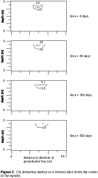

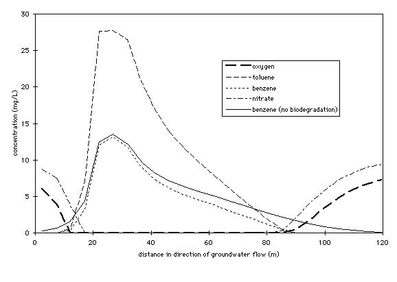
Figure 4. Concentrations of benzene without biodegradation, benzene
with biodegradation, toluene, oxygen, and nitrate in upper 1.2 m of aquifer
along aquifer center line at 500 days.
