Constructing Potentiometric Maps
When the file has
been prepared for Arcview, add it to the project with the Add
Table command located in the project window. Then
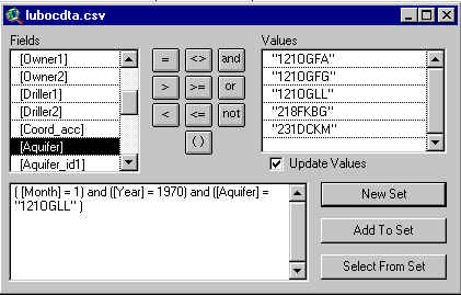
open the table and click on the query tool ![]() . Since the potentiometric surface
changes through time, the data selected from the file should
represent a short time interval. The month of January is
the most common entry date, with other months having very few
entries and in some cases none. In addition, you should
query those entries that correspond to the aquifer of interest
only, as the file will most likely contain data from more than
one aquifer ("Aquifer" field). Here is an example
query:
. Since the potentiometric surface
changes through time, the data selected from the file should
represent a short time interval. The month of January is
the most common entry date, with other months having very few
entries and in some cases none. In addition, you should
query those entries that correspond to the aquifer of interest
only, as the file will most likely contain data from more than
one aquifer ("Aquifer" field). Here is an example
query:
Now the data can be added to the view as an "event theme". When the view is active, select View/Add Event Theme. The following box should appear with longitude as the x-field and latitude as the y-field and with the name of the data file in the "Table" field.
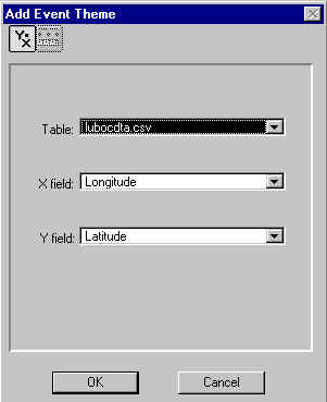
After clicking OK, you will see that the displayed data points are the same ones that were selected with the query tool. The event theme can also be converted to a shapefile with the command: Theme/Covert to Shapefile, but this is optional.
This map and those that follow will require that the projection be changed to one that has map distance units in feet or meters in order to make the selection of an appropriate cell size easier. I have chosen to use the Albers Equal Area projection, which has map distance units in meters. The projection is changed by selecting View/Properties. Then click projections, select Albers Equal Area, and click on custom. The custom projection parameters that I used are:
central meridian = -101.8
reference latitude = 33.0
standard parallel 1 = 33.5
standard parallel 2 = 34.5
false easting = 0
false northing = 0
You will have to choose projection parameters by trial and error. In general, the central meridian and referecne latitude should run through the center of the area of interest and standard parallels one and two should be 1/6 of the way from the bottom and the top of the area of interest respectively.
Now, the data can be used to create a potentiometric map. First, make sure that the extension Spatial Analyst is active. If not, make the project window active and go to File/Extensions. Then, with the view active, select: Surface/Interpolate Grid. The following box should appear:
The Output Grid Extent should be the same as your data file. The cell size and number of rows and columns are automated, although you can change these values. I have chosen to use a cell size of 1000m here.
When you click OK, the following box will appear:
You are given a choice of either the inverse distance weighting (IDW) method or the spline method for interpolating a surface. I prefer to use the IDW method because it appears to more closely honor the data. Next, select "Water_elev" as the Z Value Field. Then choose the appropriate calculation parameters. This may take some trial and error. The No. of Neighbors, or the number of nearest data points to the cell value being calculated, should be dictated by the density of the data set. The greater the density, the greater the number of neighbors. I used 6 neighbors instead of the default 12 to generate the map below. When you click OK, the surface will be generated.
Finally, go to Theme/Save Data Set and rename the new surface file. If you do not do this, Arcview automatically names the surface for you. This can create some confusion after you have generated several surfaces with generic names.
The following is a potentiometric surface generated from data from Lubbock, Lamb, Hale, and Hockley counties during January 1970. The county outlines overlaid on the map were obtained from the Texas Natural Resources Information Service web site.
Potentiometric Map
The highest water levels are in the northwest corner and the lowest in the southeast, therefore the direction of groundwater movement is towards the southeast. The map represents the potentiometric surface in the Ogallala aquifer and, in this case, the potentiometric surface is the same as the water table because the Ogallala is an unconfined aquifer. The Ogallala is a sand and gravel aquifer that was deposited by streams. The following map is a map of the Ogallala formation with the study area outlined in red.
(This image was obtained from the Texas Water Development Board publications download area)