
Constructing Potentiometric Maps
in Arcview
GIS in Water Resources Term Project, Spring '98
This report will present a procedure that I have developed to create potentiometric maps in Arcview. Arcview provides an easy-to-use interface that brings well data and other relevant features such as geology, rivers, roads, cities, ect. into a common display environment. In addition, the query tool provides a quick way to pick data of interest out of large files that would otherwise take hours to edit manually. Potentiometric maps are useful to any hydrological investigation because they help one see how the potentiometric surface appears in 3D as opposed to a point measurement at a well bore. However, the user should be cautioned that a potentiometric map drawn by any interpolation method is merely a hypothesis.
Outline
The objectives of this project are:
Develop an efficient method for the collection and preparation of Texas Water Development Board well data.
Generate a potentiometric surface map in Arcview
Determine possible applications for the wate level data and potentiometric maps.
The potentiometric surface is the level to which water rises in a well. In a confined aquifer this surface is above the top of the aquifer unit; whereas, in an unconfined aquifer, it is the same as the water table. The following cartoon depicts an aquifer with an unconfined section on the left and a confined section on the right (Fetter, 1994).
(Fetter, 1994)
As you might expect, a potentiometric map is a contour map of the potentiometric surface. As on the surface of the earth, water flows from high elevation, or potential, to low elevation. Thus a potentiometric map indicates which direction water is moving in the subsurface.
A countour map is a 2D representation of a 3D surface that is defined by a set of points having x, y, and z coordinates. The x and y coordinates correspond to longitude and latitude respectively and the z coordinate corresponds to the elevation of the potentiometric surface above mean sea level. Therefore, the data requirements of this project include well coordinates, well head elevation, and water level elevation.
I obtained the water data from the Texas Water Development Board web site. The data is located in the "Water Conditions and Data Download Area"
(click on the figures to obtain a larger view)

![]()

![]()
Next go to "Download TWDB Ground Water Data Base Files in ASCII Text Format" and you will see a disclaimer.

![]()
The disclaimer provides a description of the contents and limitations of the ground water data base. The file "Appg.txt" contains a description of the data fields that you will need to understand what is in each file because the fields are not labeled. Right click on "Appg.txt" to obtain a copy or download it from the disclaimer section. Scroll to the end of the page to find the data download area link that will take you to the ftp area.
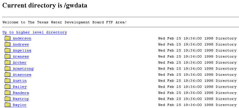
From the gwdata directory you can select the county folder of interest.
![]()
There are several files available, but the most important are aquifer.txt, wlevels.txt, and weldta.txt. Click on "aquifer.txt" to obtain a copy of the file. It contains a list of aquifer codes associated with the corresponding aquifer names that are needed to identify in which aquifer a well is screened. After selecting the county folder, copy the files: aquifer.txt, weldta.txt, and wlevels.txt.
"wlevels" contains the water depth entries and their corresponding collection dates; however, the well elevation is needed to convert the depth entries to water level elevation. Here is an example wlevels file where I have added the field labels.
Well# |
pub-or-nopub |
water_depth |
Month |
Day |
Year |
meas# |
meas-agency |
meas-meth |
remark |
4601202 |
P |
-42.7 |
10 |
17 |
1974 |
1 |
1 |
1 |
|
4601301 |
P |
-78.5 |
10 |
17 |
1974 |
1 |
1 |
2 |
|
4601301 |
P |
-74.15 |
11 |
12 |
1975 |
1 |
1 |
2 |
|
4601301 |
P |
-73 |
11 |
10 |
1976 |
1 |
1 |
2 |
2 |
4601301 |
P |
-83.65 |
11 |
12 |
1977 |
1 |
1 |
2 |
2 |
"weldta" contains the latitude and longitude coordinates of the well and the well elevation, but there are too many fields to show an example here.
Excel is the most convenient tool to prepare the files for use in Arcview. When opening a file, Excel first needs to know how the file is delimitted. The TWDB files are delimitted with a "|" character. This character is located on the backslash button. In order to select the "|" as the delimiter, click on other and type the character in the "other" box.
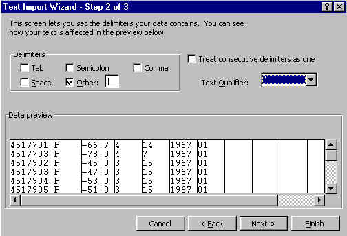
The "wlevels" and "weldta" files can now be processed, but first two obstacles must be dealt with. First, the longitudes and latitudes are in a form that is difficult to convert to decimal degrees. For example, 100 degrees, 30 minutes, and 30 seconds would be represented by the number: 1003030. The second difficulty is that the data are split into two files: "wlevels" and "weldta". These files must be merged so that the water depth field (in "wlevels") and the elevation field (in "weldta") can be added to determine the water elevation. This also simplifies the querying process in Arcview.
After spending as much as and hour preparing one 100 line file for use in Arcview, I decided to write an Excel macro that would perform all of the tasks that were necessary. This, in itself, took many hours, but the macro can now prepare an 8000-line file in approximately 30 minutes. The macro labels the data fields, converts the coordinates to decimal degrees, calculates the water level elevation, and merges the "wlevel" and "weldta" files. Click here if you would like to obtain a copy of my Excel workbook.
I developed the following code to make the conversion to decimal degrees:
'evaluate 93 degrees
If (Cells(counter, "G") > 925959) And
((Cells(counter, "G") < 940000)) Then
Cells(counter, 9).Select
ActiveCell.FormulaR1C1 =
"=(TRUNC((RC[-2]-930000)/100))/60"
Cells(counter, "H") = "93"
'calculate seconds
For counter2 = 0 To 59
If (((Cells(counter, "G") -
((930000) + (100 * counter2))) >= 0) And ((Cells(counter,
"G") - ((930000) + (100 *
counter2))) < 60)) Then
Cells(counter, "J") =
(((Cells(counter, "G")) - ((930000) + (100 *
counter2))) / 3600)
End If
Next counter2
Cells(counter, "K") = -(Cells(counter,
"H") + Cells(counter, "I") + Cells(counter,
"J"))
End If
The macro runs through a series of loops to check for those latitudes and longitudes that encompass Texas. When a match is found, it calculates the decimal minutes. Then another loop is required to calculate the decimal seconds. Finally, the degrees, decimal minutes, and decimal seconds are added. Finally, another loop searches for a match in the well number field and then copies and pastes the water depth entry from the "wlevels" file to the "weldta" file.
(Note, I will use the following notation to indicate a command that is located in a menu: Menu/Command)
After you have opened the workbook, open the "wlevels" and "weldta". Then you will have to separately move both files into the workbook in the edit menu: Edit/Move or Copy Sheet and select the workbook as the destination. If you have given them different names, then you must rename the appropriate sheets as "wlevels" and "weldta" or the macro will not recognize them. Then go to the Tools menu, then to the macros menu and finally click on macros. There you will see two macros: "latlon" and "nodata". Click on latlon to process the files as mentioned before. The visual basic script is slow, therefore you should use the fastest computer available. On a 200Mz machine, the macro processes approximately 300 lines per minute. The macro "nodata" removes all of the entries with no water depth data, but this is optional. When latlon has finished, make sure that the "weldta" sheet is active and save this sheet as a comma delimitted or *.CSV file with the command: File/Save As. Before you open the file in Arcview, you should make a note of the aquifer code of the aquifer of interest, located in "aquifer.txt".
Constructing Potentiometric Maps
When the file has
been prepared for Arcview, add it to the project with the Add
Table command located in the project window. Then
open the table and click on the query tool ![]() . Since the potentiometric surface
changes through time, the data selected from the file should
represent a short time interval. The month of January is
the most common entry date, with other months having very few
entries and in some cases none. In addition, you should
query those entries that correspond to the aquifer of interest
only, as the file will most likely contain data from more than
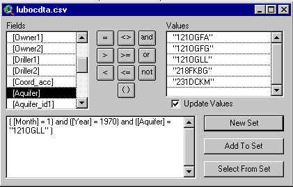
one aquifer ("Aquifer" field). Here is an example
query:
. Since the potentiometric surface
changes through time, the data selected from the file should
represent a short time interval. The month of January is
the most common entry date, with other months having very few
entries and in some cases none. In addition, you should
query those entries that correspond to the aquifer of interest
only, as the file will most likely contain data from more than
one aquifer ("Aquifer" field). Here is an example
query:
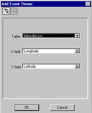
Now the data can be added to the view as an "event theme". When the view is active, select View/Add Event Theme. The following box should appear with longitude as the x-field and latitude as the y-field and with the name of the data file in the "Table" field.
After clicking OK, you will see that the displayed data points are the same ones that were selected with the query tool. The event theme can also be converted to a shapefile with the command: Theme/Covert to Shapefile, but this is optional.
This map and those that follow will require that the projection be changed to one that has map distance units in feet or meters in order to make the selection of an appropriate cell size easier. I have chosen to use the Albers Equal Area projection, which has map distance units in meters. The projection is changed by selecting View/Properties. Then click projections, select Albers Equal Area, and click on custom. The custom projection parameters that I used are:
central meridian = -101.8
reference latitude = 33.0
standard parallel 1 = 33.5
standard parallel 2 = 34.5
false easting = 0
false northing = 0
You will have to choose projection parameters by trial and error. In general, the central meridian and referecne latitude should run through the center of the area of interest and standard parallels one and two should be 1/6 of the way from the bottom and the top of the area of interest respectively.
Now, the data can be used to create a potentiometric map. First, make sure that the extension Spatial Analyst is active. If not, make the project window active and go to File/Extensions. Then, with the view active, select: Surface/Interpolate Grid. The following box should appear:
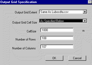
The Output Grid Extent should be the same as your data file. The cell size and number of rows and columns are automated, although you can change these values. I have chosen to use a cell size of 1000m here.
When you click OK, the following box will appear:
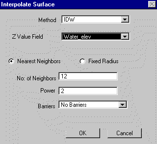
You are given a choice of either the inverse distance weighting (IDW) method or the spline method for interpolating a surface. I prefer to use the IDW method because it appears to more closely honor the data. Next, select "Water_elev" as the Z Value Field. Then choose the appropriate calculation parameters. This may take some trial and error. The No. of Neighbors, or the number of nearest data points to the cell value being calculated, should be dictated by the density of the data set. The greater the density, the greater the number of neighbors. I used 6 neighbors instead of the default 12 to generate the map below. When you click OK, the surface will be generated.
Finally, go to Theme/Save Data Set and rename the new surface file. If you do not do this, Arcview automatically names the surface for you. This can create some confusion after you have generated several surfaces with generic names.
The following is a potentiometric surface generated from data from Lubbock, Lamb, Hale, and Hockley counties during January 1970. The county outlines overlaid on the map were obtained from the Texas Natural Resources Information Service web site.
Potentiometric Map
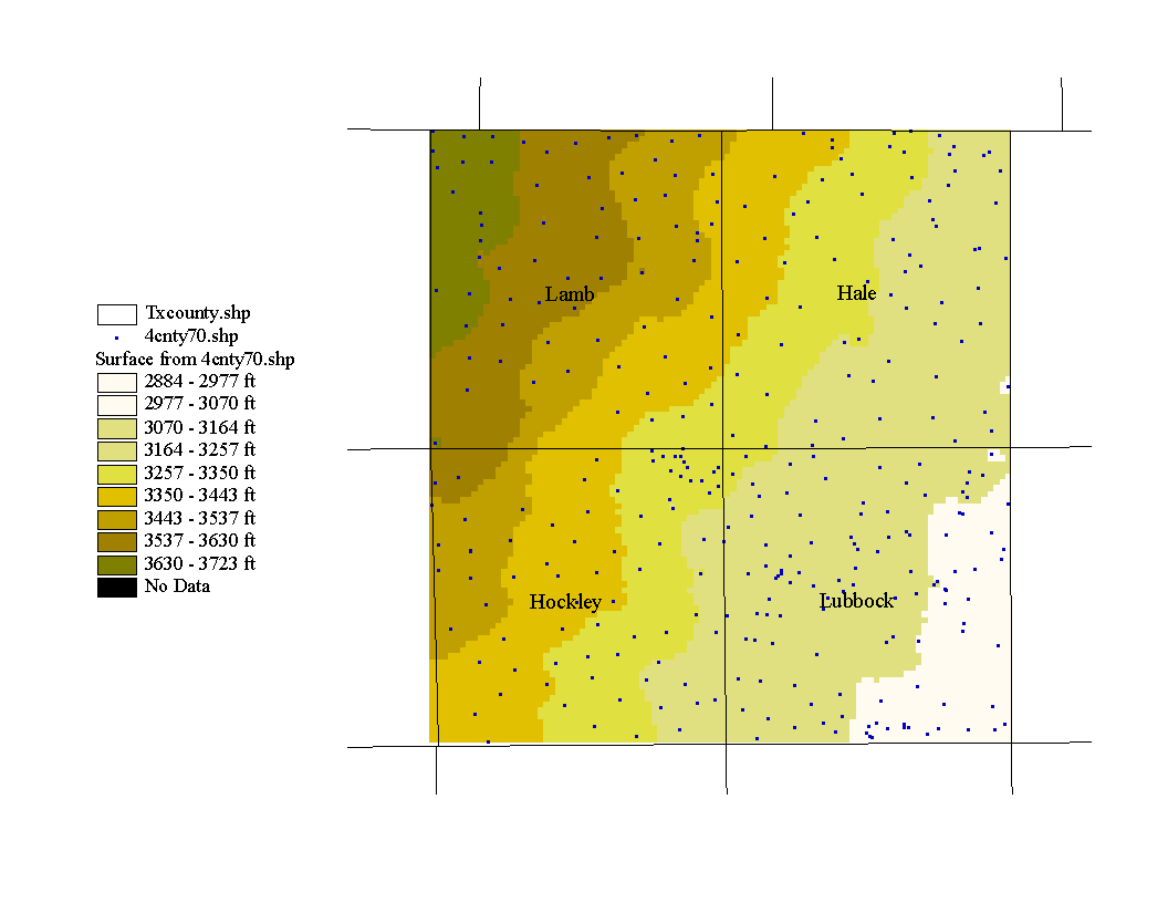
The highest water levels are in the northwest corner and the lowest in the southeast, therefore the direction of groundwater movement is towards the southeast. The map represents the potentiometric surface in the Ogallala aquifer and, in this case, the potentiometric surface is the same as the water table because the Ogallala is an unconfined aquifer. The Ogallala is a sand and gravel aquifer that was deposited by streams. The following map is a map of the Ogallala formation with the study area outlined in red.
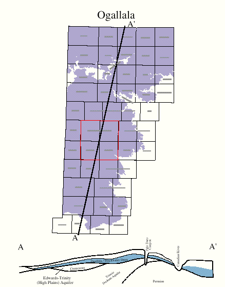
(This image was obtained from the Texas Water Development Board publications download area)
Applications for Potentiometric Maps
Potentiometric head data can easily be used to map trends in the water levels of a region and the properties of an aquifer. As an example, I have chosen the Ogallala aquifer of the High Plains, where significant groundwater declines have occured since pumping began in the 1940's.
Here is a map of net water level changes in Lubbock, Hockley, Lamb, and Hale counties from January 1970 to January 1981.
Map of Water Level Change, 1970 to 81
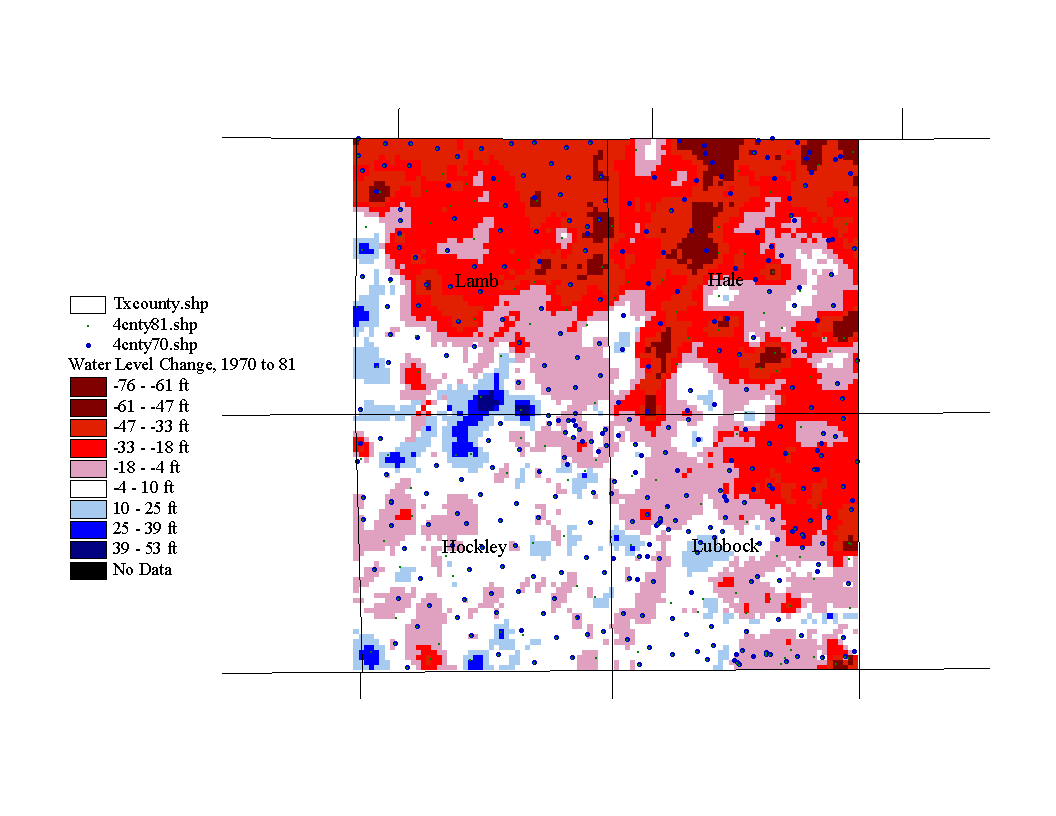
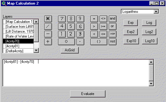
This map was generated with map calculator by subracting the Jan. 1970 potentiometric map from the Jan. 1981 potentiometric map, i.e. the water elevation value of each cell of the 1970 map was subtracted from each cell value of in 1981 map. You will find map calculator in the Analysis menu. Again, Spatial Analyst must be active in order to perform this function. Below is the map calculation that produces the above map.
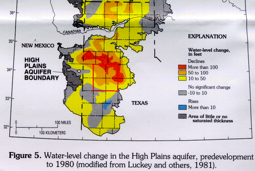
Map of Water Level Change, Predevelopment to 80
I obtained this map from the USGS Water Resources Investigations Report #95-4208, "Water Level Changes in the High Plains Aquifer-Predevelopment to 1994". Although the time period represented by the previous map is 1970 to 80, it is interesting to note that the general trends agree well. In both maps, water level declines are greatest in the northeastern portion of the study area than in the southwestern section.
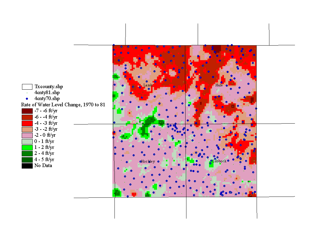
The next application is similar to the first. It is a map of the rate of water level change for the same area, during the same time period. In map calculator, the 1970 map is subtracted from the 1981 map as before, but now this quantity is divided by 11 years. Each cell now has a value that is the rate of water level change in feet per year.
Map of Rate of Water Level Change, 1970 to 81
The next application is a map of saturated thickness. Since the Ogallala is an unconfined aquifer, the water table is the upper bounding surface of the aquifer. The lower bounding surface is the contact with underlying Cretaceous and Triassic units. The thickness of the aquifer is simply the distance from the water table to the lower bounding surface of the Ogallala, but it does not closely resemble the water table map because the Ogallala was deposited on a rough surface with hills and stream valleys.
Map of Saturated Thickness, 1970
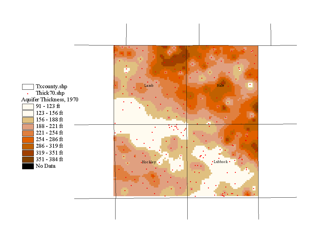
This map is merely a demonstration of the method that would be used to construct an aquifer thickness map, but probably a poor representation because the well depths were assumed to represent the depth to the bottom of the aquifer. This assumption was made because because it would have been extremely time consuming to obtain the well logs and enter the aquifer depth data by hand.
In order to prepare the data file for the thickness map, I exported the 1970 attribute file into Excel, deleted all entries without well depth data, converted the well depths to elevations, subtracted the well depth elevation from the corresponding water level elevation, and subtracted the well depth from the water elevation. Then the file was added to the veiw in Arcview and a surface was generated as before.
I initially tried to make an aquifer thickness map by generating a map of the lower bounding surface of the aquifer and subtracting it from the potentiomtric surface, but this yielded some negative values. This is probably because the well depth entries do not always represent the actual depth of the aquifer, as well as the fact that the interpolated surfaces may intersect in areas where there are few data points to constrain the interpolation.
The next application is a map of the volume of water in storage in the Ogallala aquifer during January 1970.
Map of Aquifer Storage, 1970
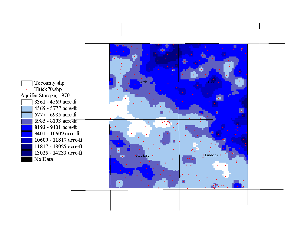
The volume of water stored in an aquifer is simply the volume of the aquifer times the specific yield. The specific yield is the drainable portion of the pore water where porosity=specific yield + specific retention. The specific retention is that portion of the pore water that is held in contact with the mineral grains and cannot be drained; thus, it is not included in the storage calculation (Fetter, 1994). Now the new map can be generated in map calculator. The calculation is as follows: (("aquifer thickness map") x (cell area) x (specific yield) x 0.3048) / 1233. You can determine the cell area by clicking on any cell with the information tool. I used a specific yield value of 15% as in Bell and Morrison, 1978. The number 0.3048 is a conversion factor from square meters to square feet. The number 1233 is a conversion factor from cubic feet to acre-feet.
Another important application is a map of the distance from the surface to the potentiometric surface, or in this case, water table. This lift distance determines how much energy is required to pump water to the surface. As the water table falls, the lift distance increases and so does the energy needed to lift the water. This means that a consequence of pumping is that the more water that is pumped, the more expensive it becomes to pump more water (Bell and Morrison, 1978).
In order to generate the following map, I first selected those data points in the 1970 well coverage that intersect the 1981 well coverage so that I could compare the change in lift distance from 1970 to 1981. The procedure for selecting intersecting data points is as follows: with the theme active go to the theme menu: Theme/Select by Theme, under select features of active theme that select intersect, under the selected features of select the file that should have intersecting features with the active theme, then in the theme menu: Theme/Convert to Shapefile. Now you can use the new theme to generate the lift map with the procedure described in the previous section "Potentiometric Map Construction".
Map of Lift Distance, 1970
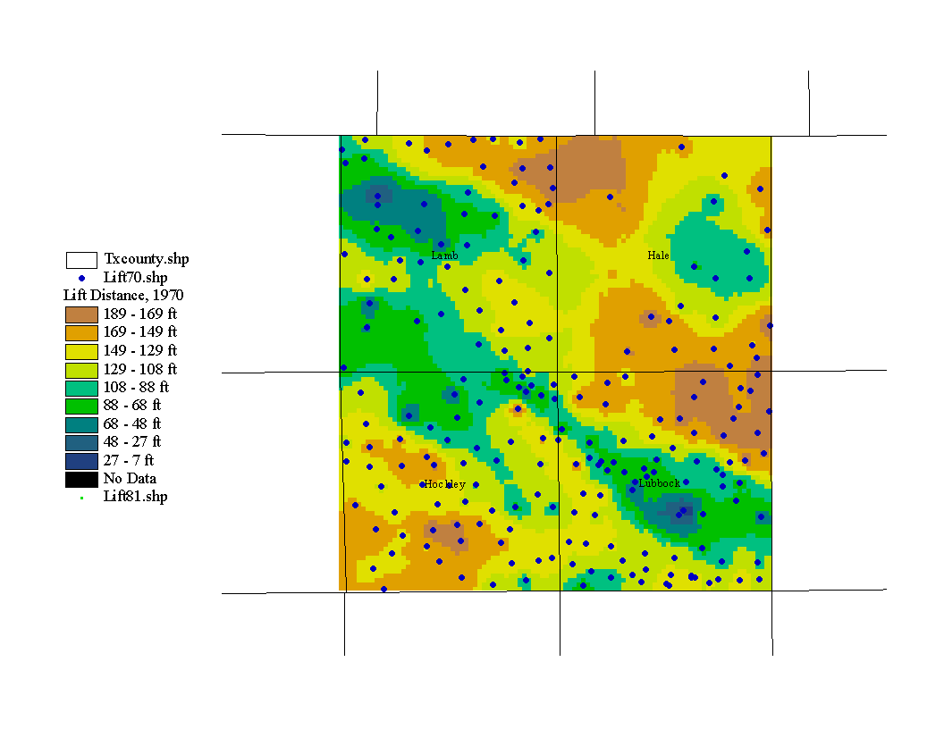
According to the above map, it should be cheaper to pump water in the city of Lubbock than in northeastern Lubbock county.
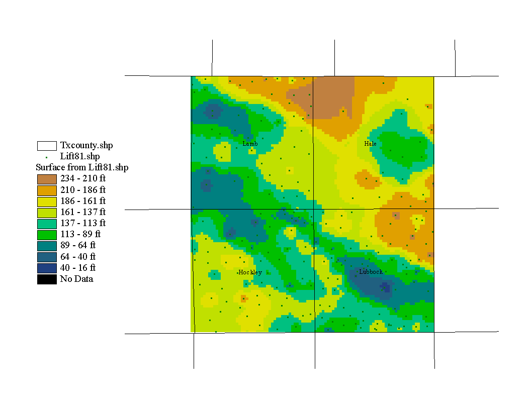
The next map is the same as the previous one except that the data set is from January 1981. As before, those data points that intersect 1970 were selected to create a new data set that can be compared with the above map.
Map of Lift Distance, 1981
The next map is the change in lift distance from 1970 to 81. It is similar the map of water level change except that it depicts the change in the lift distance and thus the change in the amount of energy required to lift water to the surface.
Map of Change in Lift Distance, 1970 to 81
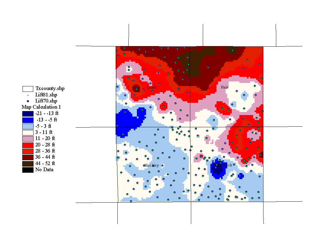
The red values represent increased lift distance and the blue values represent decreased lift distance. According to the above map, the lift has increased by up to 52 feet in the northern section of the study area, making pumping more expensive in that region.
A procedure for well data collection and preparation for use in Arcview has been developed here.
Potentiometric maps can be easily constructed using the "Spatial Analyst" extension in Arcview.
Potentiometric maps and water level data can be used to depict the current status or past trends in an aquifer.
Problems Encountered
The longitudes and latitudes in the TWDB files must be converted to decimal degrees.
The water level entries are in a separate file from the well location and elevation data that must be merged.
Where to go from here?
The process developed here should be used to predict how an aquifer will respond to pumping or climate change possibly with the available Arcview tools or in conjunction with a groundwater model such as MODFLOW.
| Data Label | Feature | Class | Attribute | Description |
| aquifer.txt | - | - | - | file containing aquifer names and corresponding aquifer codes |
| AppG.txt | - | - | - | file containing a description of what is contained in the TWDB files |
| wlevels.txt | - | - | - | contains water depth entries |
| weldta.txt | - | - | - | contains well location and elevation |
| twdb.xls | - | - | - | workbook with macro that prepares wlevels.txt and weldta.txt for Arcview |
| county.shp, .dbf, .shx | counties of Texas | arc | county names | - |
| 4county70.csv | well locations | point | well data: | event theme: well data for Lubbock, Hale, Hockley and Lamb counties for January 1970 |
| Well# | 7 digit well identification number | |||
| Pub_NonPub | publishable/nonpublishable | |||
| Water_Depth | depth to water from top of well casing | |||
| Water_Elevation | elevation of potentiometric surface | |||
| Month | month of data collection | |||
| Day | day of data collection | |||
| Year | year of data collection | |||
| Measure# | measurement number | |||
| Meas_Agency | measurement agency code | |||
| Meas_Method | water level measurement method code | |||
| Remarks | miscellaneous remarks codes | |||
| FIPS | FIPS county code | |||
| basin | basin code | |||
| zone | zone code | |||
| region# | region number code | |||
| previous_id | previous well identification code | |||
| Longitude | longitude coordinate of well | |||
| Latitude | latitude coordinate of well | |||
| owner1 | owner name | |||
| owner2 | owner name | |||
| driller1 | driller name | |||
| driller2 | driller name | |||
| coord_acc | coordinate accuracy code | |||
| aquifer | primary aquifer identification code | |||
| aquifer_id1 | aquifer identification code | |||
| aquifer_id2 | aquifer identification code | |||
| aquifer_id3 | aquifer identification code | |||
| surf_elev | surface elevation | |||
| elev_meas | method of elevation measurment code | |||
| users_econom | users' economics code | |||
| date_drilled | date that well was drilled | |||
| well_type | well type code | |||
| well_depth | depth of well casing | |||
| depth_meas | method of depth measurment code | |||
| lift_type | lift type code | |||
| power | lift power type code | |||
| horsepower | pump horespower | |||
| primary_user | primary well user code | |||
| second_user | secondary user code | |||
| third_user | tertiary user code | |||
| levels_avail | water levels available in TWDB files (C,H,M,R,N) | |||
| water_quality | water quality data available (y/n) | |||
| log_avail | well logs available | |||
| other_data | other data available code | |||
| updated | date of data entry | |||
| agency | reporting agency | |||
| schedule_in_twdb | well schedule in TWDB files (y/n) | |||
| construction | well construction method code | |||
| completion | well completion code | |||
| casing | casing type code | |||
| screen | screen type code | |||
| lith_log_type | lithological log type | |||
| interpreter | lithological log interpreter initials | |||
| interp_date | date of lithological log interpretation | |||
| 4county81.csv | well locations | point | same as above | event theme: well data for Lubbock, Hale, Hockley, and Lamb counties for January 1981 |
| 4count70.shp, .dbf, .shx | well locations | point | same as above | 4county70.csv converted to a shapefile |
| 4county81.shp, .dbf, .shx | well locations | point | same as above | 4county81.csv converted to a shapefile |
| Thick70.shp, .dbf, .shx | well locations | point | same as above | all entries with no depth data were deleted, aquifer thickness column added |
| Lift70.shp, .dbf, .shx | well locations | point | same as above | data for points that intersect 4county81.shp |
| Lift81.shp, .dbf, .shx | well locations | point | same as above | data for points that intersect 4county70.shp |
| *.adf | - | raster | - | grids from point shape files |
Bell, A. E., and S. Morrison, Analytical Study of the Ogallala Aquifer in Lubbock County, Texas, Texas Water Development Board, Report 216, June, 1978.
Fetter, C. W., Applied Hydrogeology 3rd Ed., Prentice Hall, Inc., 1994.
Dugan, J. T., and Sharpe, J. B., 1995, Water Level Changes in the High Plains Aquifer-Predevelopment to 1994. USGS Water Resources Investigations Report 95-4208.