Term Project

Conversion of Cell-Based GIS Hydrologic Models to HEC-1 Utilizing BYU's WMS

by Dean Thomas

Table of Contents

Term Project Introduction/Overview

WMS Exercise

Conclusions

Thanks and Acknowledgements

Data Dictionary

Introduction and Overview of Term Project

I'm a believer. GIS based hydrologic modeling is here. It is no longer merely a vision of possibilities and potentials. Once it was the land of arcane command line processing, super expensive hardware, and hard to obatain data with limited applications. Today, GIS hydrology is a PC, GUI based reality with ever-increasing availability and quality of data. Not to get too dramatic, but I seriously believe we are on the verge of a revolution in the way hydrology is studied and modeled in mainstream engineering. The benefits of GIS based hydrology are overwhelming, with limitations that become smaller each day. While the technology is constantly evolving and improving, it must be satisfying for those whose vision and hard work has brought the technology to fruition.

Well, okay, if everything is so great, why does this paper need to be written? In a word, credibility. New technology is almost never immediately accepted in the mainstream. Of course, this is a good thing, resulting in the weeding out of inaccurate and flawed methodologies. Although GIS based models have been demonstrated to provide accurate results (with proper usage), until the technology reaches a level of mainstream acceptability its usefulness will be limited for commercial application requiring approval of regulatory agencies. Those unfamiliar with the technology naturally generally harbor a skeptical attitude about the accuracy of GIS based models.

In addition, having a "base-line" model or a known technology makes for a quick check of the accuracy of new technology. Regardless of the acceptance of the new model by others, those involved in the development will want to make it as accurate as possible. Where differences arise, there may be logical explanations for the discrepancies. But it is reassuring to have a sense that a new algorithm or program is representative of the physical processes modeled.

Considering the above, a link between existing proven models and GIS based models would appear to be a handy tool. The GIS sofware most utilized by Dr. Maidment and the researchers at the CRWR at UT are Arc/Info and ArcView from ESRI. These software packages do not offer an interface, or standard method, to migrate GIS, and especially  raster data, to a "traditional" lumped sum hydrologic computer model such as HEC-1 or TR-20. Enter the "Watershed Modeling System" (WMS) GIS hydrologic software package from the BYU Engineering Computer Graphic Laboratory. In addition to its own GIS capabilities, WMS is designed completely for spatial hydrologic modeling. The software GIS data to be used to create a variety of  "industry standard" models, including HEC-1. WMS also allows the user to run HEC-1 from within WMS, as well as check the input file for errors. An excellent graphics system and post processor capabilities are also included.. This is the link I'll use to demonstrate how to move cell-based digital data created in the Arc environment to a standard HEC-1 model. The resulting HEC-1 model will then be compared to existing studies to see if the parameters and results are reasonable.

The paper will explain certain WMS features, but by no means covers the capabilities of the program. Interested readers are encouraged to explore WMS (they even have a free download demo version and complete manuals!) for a better understanding of the software and the possiblities it provides the user.

The watershed used for the study is the Barton Creek watershed area near Austin, Texas. The data is in Arc/Info grid format with 30 meter resolution. One problem with existing GIS raster data is that the resolution is not sufficient for urban studies. This paper utilizes 30 meter data cell grids that were processed in Arc/Info and are available thanks to Christine Dartiguenave. For those interested in using GIS in urban areas, Christine's research should prove quite helpful.

Return to Table of Contents

WMS Exercise: Converting Arc/Info Grids to an HEC-1 input file using WMS

Goals of the exercise

The purpose of this exercise is to demonstrate how to convert Arc grid data to a format usable by WMS, and create an HEC-1 input file.

Computer and Data Requirements

This exercise utilizes Arc/info with the Grid module, and the pc version of WMS beta 5.0. Please note, as of this writing, version 5.0 is not commercially available, and is considered to be in the development and testing stage.

Data needed:

This exercise can be performed with the following data:

• A dem in Arc/Info grid format
• A flow direction grid in Arc/Info format
• A flow accumulation grid in Arc/Info format

Be sure that your grids are correctly projected, as WMS does not offer projection capabilities. Each grid must also have the exact extent of coverage. For my paper, I used the following grids:

• barton_dem(30 meter elevation grid)
• barton_fdr(30 meter flow direction grid)
• barton_fac(30 meter flow accumulation grid)

All the grids are in Arc/Info format, which means that they may have been processed in Arc/info or in ArcView with Spatial Analyst.

Procedure

1. Converting the data

If you need help on how to get to your Arc/Info or ArcView data to this point and ready for conversion, check out exercise 2 or exercise 6 from Dr. Maidment's GIS in Water Resources class at The University of Texas. Otherwise, it is assumed the dem, flow direction, and flow accumulation grids have been created. As with any computer generated information, verify that the results are representative of the physical system.

Now we're ready to convert our grid files to ASCII text files that can be read by WMS. Crank up Arc/Info (whether the grids were created in ArcView or Arc/Info). The command gridascii is used from the arc prompt, with the following usage:

gridascii <ingrid> <outfile> {item}

where item is the cell content to be transferred. The default is the value of the cell, and so the item is not required input for this case. The command will generate a text file and a projection file. The projection file is not needed by WMS. Create a text file for the dem, flow direction, and flow accumulation grids.

2. Import the DEM

Remember, I'm only demonstrating the functions in WMS that need to be used in order to accomplish the goals of this exercise. WMS contains a comprehensive environment for hydrologic analysis, and is capable of much more than is described here. The steps shown are for the pc platform, but WMS is available for UNIX machines as well. Also, the commands to import grid data are a part of the new version not yet available. The current WMS version can import shape files for use as feature objects in hydrologic analysis.

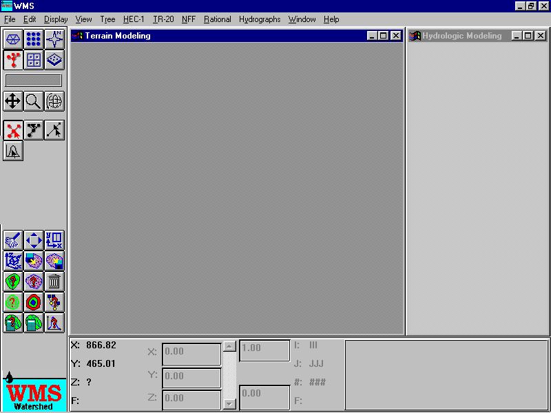
Allright, lets launch WMS. Double click on the WMS icon (or click the Watershed Modeling System icon in the WMS directory of the programs menu in Windows 95), and the following screen will appear:

In the upper left hand corner are six buttons called "modules." The tools (beneath the modules in the middle of the screen) available for use in WMS depend on the module selected. Click between different modules and see what tools are available. In the lower right hand corner of the screen a help window describes the feature currently under the mouse cursor. For most of this exercise, we will be using the DEM module, which is in the center of the top row.

Click on the DEM module, then from the File menu, choose Import. A pop-up box appears with options for importing data of differing types. Select Arc/Info grid to DEM, and click OK. Pick bar_dem.txt (or your dem grid converted to text format) and select OK. WMS reads the text file, and displays the dem contours in the graphical modeling window on the screen.

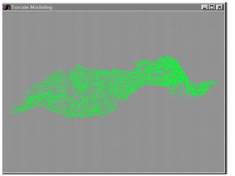
The coordinates of the image are shown in the Edit window (directly beneath the graphical modeling window). Move your mouse over the dem and you can see the elevations at each point. If you'd like to look at the dem in more detail, there are some very cool options under the Diplay and View menus, such as color ramping and changing the angle of view. To zoom in or out, use the magnifying glass icon (holding the shift button while clicking the icon zooms out). Experiment a bit and have fun.

3. Import the Flow Direction Grid

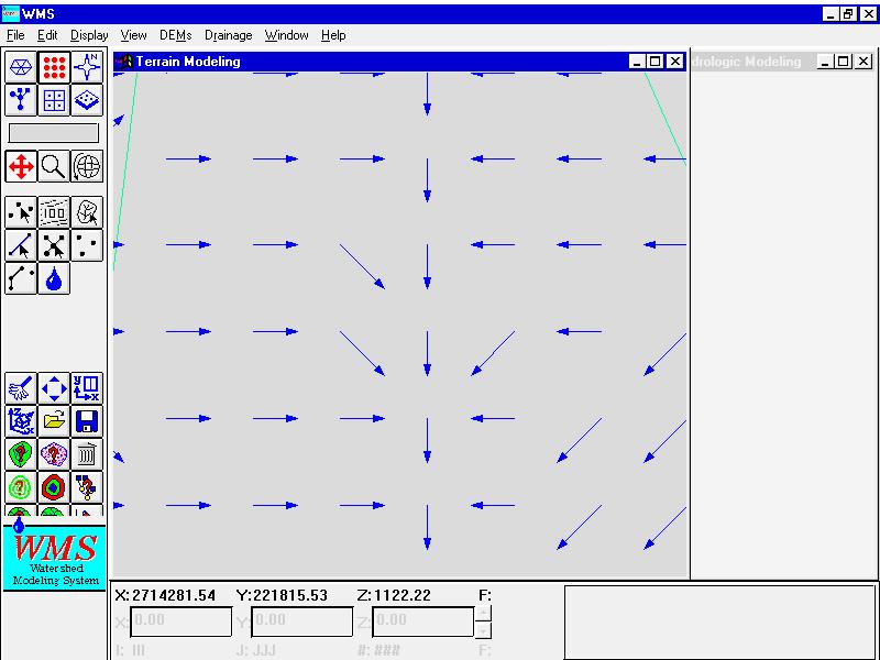
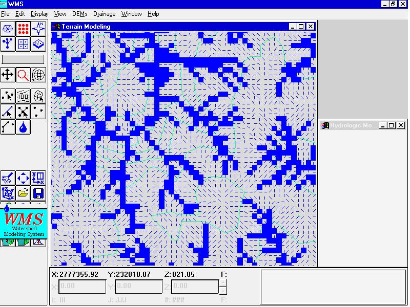
If you changed the options for the display of the dem, choose Plan View from the View menu before proceding to the next step. Make sure you still have the DEM module selected. From the Drainage menu, select Flow Directions. When the pop-up window appears, pick the Flow Direction mask and Arc/Info as the type and click OK. Select bar_fdr.txt(or your flow direction grid in text format), and hit OK. Now, depending on the resolution of your grid, this may take several minutes. Be patient, a lot of crunching is going on here. When completed, the grid appears to be a solid cover over the area.

Now use the magnifying glass icon and zoom in on a small segment of the grid. You need to zoom in very close for higher resolution grids to see that the program has actually placed an arrow indicating the direction of flow for each grid. The bar_fdr.txt grid is so dense it appears to be a solid color! By following the arrows, you can see them following the contours and eventually forming what will be the streams. Pretty cool!

4. Import Flow Accumulation Grid

Okay, so far so good. For this step, go to the Drainage menu and select Flow Directions again. This time, set the mask to Flow Accumulation and the file type again to Arc/Info. Select bar_fac.txt as the file to import, and click OK. The flow accumulation can take several minutes also, depending on your grid resolution and the extent of the grid. As an aside, if you choose Flow Accumulation from the Drainage menu, WMS will compute the flow accumulation from the dem and the flow direction grid, rather than reading in the Arc grid. Whle I don't think it really affects the results using either method, since we have consistently generated data in Arc format, we may as well use it. If you zoom in on the flow accumulation, you will see stream networks beginning to form.

5. Define Stream Network

Now things get a little more tricky. Remember that in the left middle portion of the screen there are some tool icons? Find the one that is called "Create an outlet point." Look in the help window to make sure you are selecting the right tool, and be sure you are still in the DEM module. The outlet tool icon looks like this:

Zoom in with the magnifying glass (its easiest to create a window to zoom to by clicking one corner, holding down the mouse button, and dragging to the other corner) to the point where you want your stream network to begin (the basin outlet grid cell). Select the outlet point tool, and click in the grid cell where you want the stream network to start.

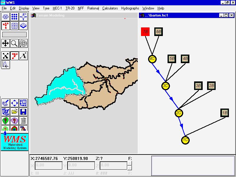
When you click on the cell for your outlet, notice that the hydrologic modeling window in the lower right of the screen has started creating a "tree model" of the watershed. This is the start of the HEC-1 input file. WMS operates mainly on feature objects. The outlet point is the first feature object we have created.

Now zoom back out by selecting Plan View from the View menu. Next, select the DEM Streams - Feature Arcs command from the Drainage Menu. Select both the Display Stream Feature Arc Creation and Use Feature Points to Create Streams options. You must also assign a threshold value to determine the minimum flow accumulation at a cell for which a stream will be created. I chose a value of 10,000, but you will need to consider the objectives of your modeling effort before selecting this number. Click OK, and watch the stream network form on the screen.

Notice in the Hydrologic modeling window a basin has been added. We now can add sub-basins to the watershed, if desired. Go from the DEM module to the Map module (the Map module icon is just to the right of the DEM module and looks like a North arrow). We'll be using the Select Feature Point tool located in the middle left of the screen. Its icon looks like this:

Select the outlet points for all sub-basins that will have an HEC-1 basin ID. At the intersection of streams, WMS has placed a red dot. Zoom in at points where you want to create an outlet for a sub-basin, use the Select Feature Point tool, and click directly over the red dots. Be sure to hold the Shift key down when selecting multiple sub-basins, or WMS will only recognize the last one input. Once all the sub-basins are selected, go to the Feature Objects menu and select Attributes. Select Draiange Outlet and OK. All the points are converted to drainage outlets, and become feature objects.

6. Define Basin

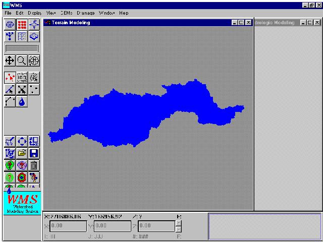
Return now to the DEM module, and from the Drainage menu select Define Basins. The extent of the drainage areas are computed from the flow direction grid and outlet points. Once the process is finished, select the DEM Basin Boundaries - Polygons command from the Drainage Menu. This command creates WMS feature arcs of the watershed and sub-basin boundaries.

Now one more time into the Drainage Menu, and select Compute Basin Data. Areas of sub-basins, slopes, flow lengths, and other parameters are automatically created in this step. The Hydrologic Window will now look something like this:

We're almost home now!

In order to complete the HEC-1 input file, go to the Tree Module (lower left of the bottom row of modules).

Select the HEC-1 menu, and double click on the most upstream sub-basin. The following input file will appear, and you can edit the HEC-1 input file on-screen, using generated spatial parameters automatically inserted by WMS, and adding precipitation and some routing data. Currently, WMS computes basin area, and is able to compute lag times for unit hydrograph generation.

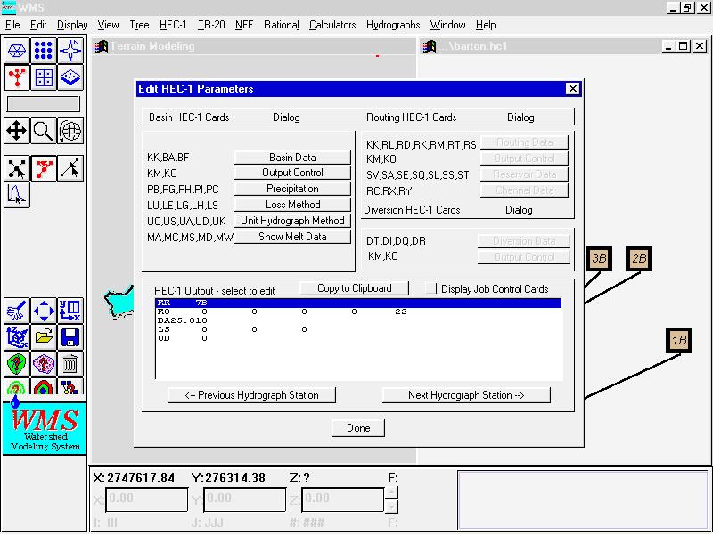
When the first basin is complete, click on the Next Hydrograph Station button, and continue to edit the HEC-1 file.

Once the HEC-1 input is done for the watershed, go to the HEC-1 menu and choose Job Control. Set the normal computational parameters for your HEC-1 run, and then again from the HEC-1 menu choose Check Model. The model checker will read the input file andl tell you if it finds any errors. Nice. This is a good point to save the files. The current beta version 5.0 of WMS cannot save imported grid data, but can save the HEC-1 file. Go to the File menu, select Save As and you will be prompted for a file name. HEC-1 input files are given the extension .hc1, output files are .out, and hydrograph Tape 22 files are given an .sol extension. If everything seems okay, from the HEC-1 menu choose Run HEC-1. A DOS window will appear and HEC-1 will run. Choose OK to exit this window when prompted. You now have a standard HEC-1 output file created, as well as a Tape 22 file for hydrographs. To look at the hydrographs, go to the Display menu and choose Show Hydrograph Window. From the Hydrographs menu, select Open. Choose the file you named as your HEC-1 Tape 22 file and click OK. Small hydrographs will appear on the map at all locations where hydrographs were computed. To see the hydrograph in the Hydrograph Window, simply click on it.

Return to Table of Contents

Conclusions

WMS computed the area of Barton Creek as 108.54 square miles, while the existing FEMA study computed a watershed area of 110.3 square miles, a difference of approximately 1.5 percent. The hydrologic input for the existing study was unavailable, so I was unable to compare peak flow rates between the two models. Stream delineations in the model were very good representations of the actual stream locations, and several lag times were computed by hand for sub-basins and found to be close to those computed by WMS. Future work that I would like to perform includes using a basin with known input parameters for an HEC-1 model, to compare peak flow rates with those generated by WMS.

In looking at the software itself, WMS provides a fairly straght-forward way to migrate hydrologic data from Arc/info (or ArcView) to a standard HEC-1 input file. The software is still in the beta stage, and naturally has some bugs to work out. The program would crash or lock up at times, but some of this I attribute to the density of the grids used. Also, the generation of some of the geometric parameters has not yet been implemented in the beta version, so it is basically computing sub-basin areas and lag times, setting up the skeleton of an HEC-1 input file. Also, not being able to save the import grid files means each time the data is worked on, every one of the steps above had to be recreated. Another area I hope to see integrated into WMS would be the ability to compute curve numbers from grid based land use and soil data. If this feature were to be put in place, an HEC-1 input file could almost entirely be created automatically from raster based data (WMS supports this feature in vector form at this time). The time savings of such an application would be enormous, and I can imagine demand for software with such an application would be high.

On the brighter side, the software was fairly intuitive, has a nice user interface, and an excellent environment for pre and post processing of HEC-1 data. Another nice feature is the ability to display scanned images or maps on the screen behind the GIS data. This gives the viewer a better feel for locations and area. For presentation purposes, text and annotation can be inserted onto the images, and much of the text (basin id's, area, etc) can be automatically brought onto the screen. On the whole, the package is extremely nice as a complement to the HEC-1 model. The results can be presented along with very nice graphics, creating a well rounded model.

The use of GIS in hydrologic modeling is so logical and time saving it cannot help but become a more dominant technology. As the use of these models becomes more wide-spread and better understood, the more they will be accepted as a standard methodology. I believe that commercially available GIS hydrologic models will be accepted within the next few years on their own merits, without having to show similar results to an existing industry standard model each time. For that reason, I don't think its necessary for every GIS software that can perform hydrologic modeling to create its own interface to HEC-1 et al. The real need is for a way to demonstrate that GIS can perform as well as (or better) than traditional models, a role that WMS can perform very well.

Return to Table of Contents

Thanks and Acknowledgements

Mucho kudos to Norman Jones at BYU for allowing me to use the Watershed Modeling System for this paper, and giving me the latest beta version for the importing of the Arc/Info grid files. I am also grateful to Chris Smemoe of BYU for his quick responses to my countless questions over the last three months. And of course thanks to Dr. Maidment, who ran a lot of interference for me in obtaining the programs and data, and kept me on track (most of the time).

Return to Table of Contents

Data Dictionary

Return to Table of Contents