Goals of the Exercise
Computer and
Data Requirements
Procedure
1.
Statistics of the Data
2.
Frequency Histogram
3.
Exceedance Probabilities
4.
Standard Error of the Mean
5.
Difference in Means Between two Data Sets
The first step in many environmental risk assessments is to collect some samples and analyze to see if the ambient concentrations of a chemical are sufficiently high to cause concern. The data used in this example are values for Benzene in soil in ug/kg (micrograms of Benzene per kilogram of soil) as measured at the Marcus Hook Refinery in Pennsylvania. The data were extracted from an Access database of data measured at the site using a procedure developed by Andrew Romanek. The presence of Benzene indicates a leakage of gasoline type fluids and the presence of nonaqueous phase liquids (NAPL) in the soil. The first step in statistical analysis of data is the determination of the statistics of the data and a characterization of its probability distribution. Once these items are known, the probability that the observed levels of the chemical exceed an acceptable level can be determined.
1. To perform a basic statistical analysis of an environmental chemical data set using MS Excel
2. To study the frequency distribution of the data and attempt to determine its probability distribution
3. To determine the probability that a sample taken randomly from this distribution will have a concentration exceeding a threshold level of concern.
4. To look at the properties of the mean of the sample as the number of data values increases. How much data is enough?
Computer and Data Requirements
This exercise requires use of a spreadsheet program or other package by which statistical functions can be performed. This description assumes the use of MS Excel Version 7.0. The data are contained in a .xls format for MS Excel 7.0 or in a .txt format (tab delimited text) for as file MHRsoil on the Learning Resource Center Server at \lrc\class\maidment\risk. The files can be downloaded from here: MHRSoil.xls or MHRsoil.txt.
The first thing one does with a new data set is to calculate its statistics, such as its mean, median, standard deviation, coefficient of skewness and the range. These values summarize the mipoint of the data, its spread around that midpoint, the symmetry of that spread, and the difference between the largest and smallest values. When the data are highly skewed (mean is >> median), then the logarithms of the data may better summarize its statistical characteristics. You can get see the names that Excel gives to particular functions by looking in the Insert menu under Functions.
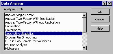
Copy the 90 data values in the data set into a new Excel spreadsheet for analysis. Under MS Excel 7.0, in the Tools menu option, choose Add-Ins. In the analysis options available, choose Analysis ToolPak. This results in a new item called Data Analysis, and the bottom of the tools menu. Selecting this option opens a tool window. Choose Descriptive Statistics from this window to get a range of statistical measures of the data. You'll see that the raw data have a very large range but the logarithms are better behaved.

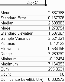
The result for the logarithms of the data looks like this:
(1) To be turned in:
(a) Descriptive statistics of the original 90 data values. What is the range of the data? What is the value of the mean compared to the median. What is the coefficient of skewness? What do these values tell you about the distribution of these data?
(b) Descriptive statistics of the logarithms to base 10 of these data. Look at the coefficient of skewness and the value of the median compared to the mean. Are logarithms or raw data a better representation of these sample values?
Under Analysis Tools, select Histogram. Make sure the Cumulative Percentage and Chart Output boxes are checked and that you enter a Bin range as well as a data range. The Bin range permits you to specify the intervals into which the data will be divided. In the example shown below for logarithmic data, the bin range divides the data by unit intervals of logarithms or by powers of 10 in the raw data.

The resulting histogram in the log space looks like this:
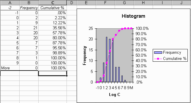
You can see that the logarithms of the data are fairly close to being symmetrically disributed (i.e. normally distributed in the log space) but there is still some assymetry in the distribution. A more complex analysis would seek to represent this assymetry using the Log Pearson Type III distribution. If we were seeking to characterize the likelihood of exceeding threshold concentrations near the ends of the distribution, that analysis may be worthwhile, but lets not pursue that for now.
(2) To be turned in: A copy of the histogram of the logarithms of the data.
Note: to do a screen capture on a PC, use Ctrl-Print Screen
to copy the contents of the screen onto the clipboard, then open the Paint
program in the Accessories menu of the PC (not in Excel).
Select Edit/Paste to get the image pasted into Paint, then use the
box select tool ![]() to draw
a box around the portion of the screen capture that you want to retain.
Use Edit/Copy To to save this file as a .bmp file. You can
then then import it into Word as an image. If you want to put the
file into an html document, open the .bmp file using Lview and save
the file in .gif format.
to draw
a box around the portion of the screen capture that you want to retain.
Use Edit/Copy To to save this file as a .bmp file. You can
then then import it into Word as an image. If you want to put the
file into an html document, open the .bmp file using Lview and save
the file in .gif format.
Lets suppose we want to know what is the chance that a sample taken randomly from the soil at the Marcus Hook refinery has a benzene concentration that exceeds a threshold level of 1,000, 10,000 or 100,000 ug/kg. Since these values lie within the range of the available data, we can do this by doing a frequency analysis of these data. First, order the data from largest to smallest, and assign a rank number to each data value, beginning with the largest value has rank m = 1, the next largest has rank m = 2, and so on. The top of the table will appear as:
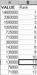
There are n = 90 values in this data set. The probability that the random variable C exceeds a value c* is estimated by counting the number of values satisfying that criterion in the data set and dividing the result by n+1, thus:

Hence, if c* = 100,000 ug/kg, the resulting probability is
P(C>100,000) = 11/91 = 0.121
Obviously the precision of this method improves as the size of the data set increases. There is always an issue in measuring environmental data as to when has enough data been collected. To get some feeling the variability inherent in the data set, do the following:
(3) To be turned in:
(a) Determine using all 90 data values the chance that a sample will exceed 1,000, 10,000 or 100,000 ug/kg
(b) Select 30 values from the original 90 in some arbitrary or random manner. Repeat the calculation in (a) using this reduced data set.
(c) Select 60 values from the original 90 and repeat the calculation again.
(d) Compare the three sets of values for the exceedance probabilities.
Are they converging towards consistent values as the data set gets larger?
One situation where the relationship between the number of data and the precision of the result is well defined is when a sample estimate is being made of the mean, especially when the data are normally distributed or nearly so. Since the logarithms of our data are nearly normally distributed, lets do this study using them. Under normal circumstances, the mean or average of a data set is calculated as:

or

so this equation can be rearranged to give the value of the mean computed with n data as a function of that computed with n-1 data as:

You can see that as the number of data increases, the increment in
information added by each new data value diminishes. If the standard deviation
of the n data is denoted by Sn , it can be shown that if the
data samples are statistically independent of one another and a large number
of data values are taken, then the Standard Error of the Mean (like a "standard
deviation of the mean") is given by:

This equation shows that the mean of a random variable is itself a
random variable, which possesses its own set of statistics. Any function
of a random variable is itself a random variable. This equation says
that the standard deviation of the mean decreases with the square root
of the number of data value, that is, if you have four times as many data,
you will halve the uncertainty in the estimate of the mean. These
equations give us a way of quantifying the variability in the mean and
how that diminishes as the number of data increase. Lets take a look at
that with our data set. The values of the cumulative mean and the
standard deviation are calculated with the Excel functions AVERAGE
and STDEV, respectively. It is best just to use the simple
formula for the average rather than the recursive one since the recursive
one is more difficult to compute and they both give the same result.
A rough estimate of the 95% confidence limits on the mean is given by the
mean value plus or minus two times the standard error of estimate of the
mean, here symbolized by (m-2sd, m+2sd).
It is particularly important that calculations with this data set be done with the logs rather than with the raw data because the average and the standard deviations of the raw data would be dominated by the few very large values in the data set. That is not so when the logs of the data are taken. Here is a sample of the calculations for the first few values in the data set:

The result of this calculation done on all the logs of the data is graphed
as:
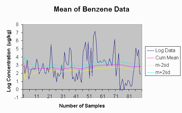
from which it can be seen that there isn't much reduction in the accuracy of the mean after about the first 30 values have been determined. There are some order of magnitude variations in the data values as shown by the wide swings in the logs of the data as the series progresses. Most likely these variations are functions of location on the site. In a later exercise, we'll plot a map of the concentrations and examine these issues more closely.
(4). To be turned in: Do the above analysis on the first 30 data values in the data set.
It often happens that one wishes to determine whether one set of environmental
data is different from another. For example, this situation arises
when comparing concentrations in wells which are upgradient from a site
and downgradient of a site. The quickest way to check that is to
determine if their mean values are different. This is done using
a t-test. Suppose the two data sets are described by the variables
x and y, which have n and m data values, respectively. The
t statistic is determined as:
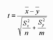
where S is the standard deviation of the data set. This formula
assumes that the standard deviations of the two data sets are approximately
equal. The test of the hypothesis that the means of the two samples
are equal is rejected if the computed value of the t-statistic exceeds
a value depending on the degree of confidence desired in the test, and
the number of degrees of freedom in the data (n+m-2), see Handbook of Hydrology
p. 17.23 for details. As an approximate measure, the two means are
different if |t| > 2, in other words if t < -2 or t > 2. These
values correspond to +/- 2 standard errors around the mean as discussed
earlier. If |t|<2, the means of the two data sets are not considered
different so the two data sets cannot be statistically distinguished from
one another.
(5) To be turned in: Compare the mean of the first 45 data values with that of the second 45 data values and determine if they are statistically different.
Return to the Class Home Page