To run the model for Waller Creek, a basin file is needed to specify the physical parameters of the watershed, and a map file to give the outline of the drainage areas and creeks. These files can be downloaded from here: Waller_Ck_1.basin and hms.map These files can also be obtained on the /class server in the LRC under /class/maidment/gishydro99/hmsintro, and also can be downloaded as a zip file: waller.zip. Make a working directory on your computer and download these files into it.
Start/Programs/hms
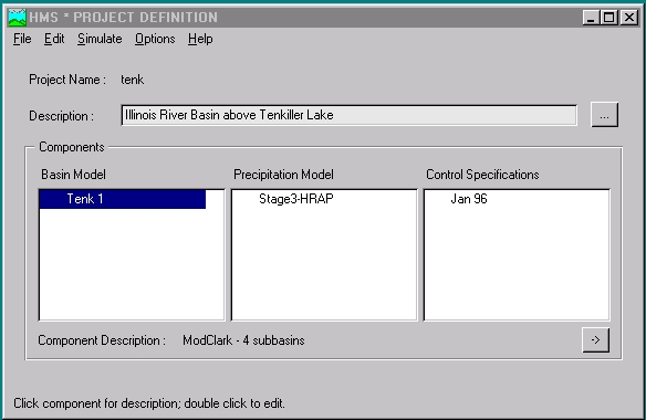
After a few seconds, a window similar to the following image should appear:
Henceforth, this image will be referred to as the Project Definition. A Project in HMS refers to all of the data sets associated with a particular model. In this case, the Project is called tenk, which is short for Lake Tenkiller. This data set is distributed as a standard example file with HEC-HMS. The Description bar underneath the Project name allows you to type a detailed name for the actual short Project name. If desired, you may click on the ellipsis to the right of the Description bar, and additional space for you to type a lengthy Description will appear. For future reference, any time you see an ellipsis in a window in the HMS, it means you may access additional space for writing descriptive text.
In the Components section of the Project Definition, there are three sub-sections--the Basin Model, the Precipitation Model, and the Control Specifications. Each component represents a different element of the model. The Basin Model, for instance, contains information relevant to the physical attributes of the model, such as basin areas, river reach connectivity, or reservoir data. Likewise, the Precipitation Model holds rainfall data. Finally, the Control Specifications section contains information pertinent to the timing of the model such as when a storm occurred and what type of time interval you want to use in the model. Each of the sections is explored below individually.

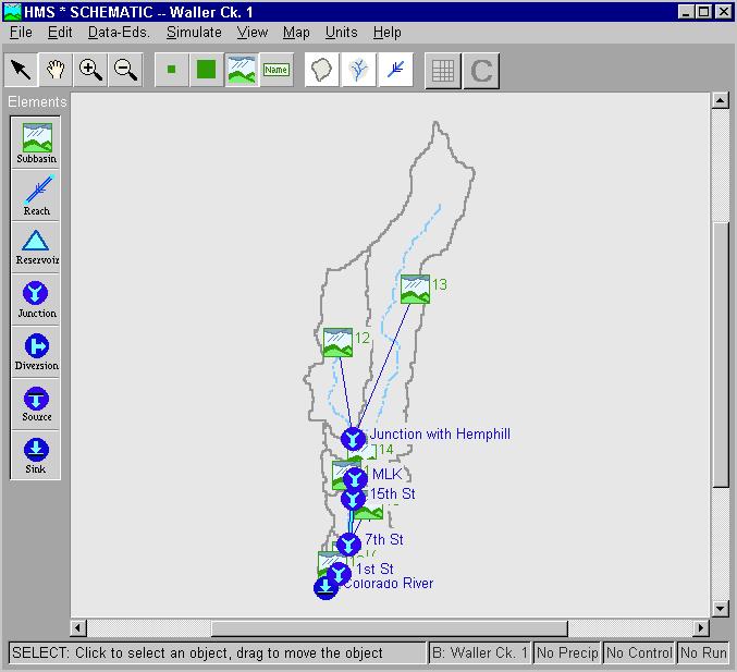
In the HMS Project window, use Edit/Basin Model/Import to import the basin model from the directory c:\temp\working. You'll see the Basin window open up and some icons appear. You may be asked for the location of the map file. In this case, in the HMS Schematic window, use File/Basin Model Attributes to select the location where you have stored the map file. You should now see a schematic of Waller Creek showing the watershed and stream map and an overlay of the hydrologic elements.
The tool bar on the left hand side of the display shows the seven hydrologic elements contained in HEC-HMS. They are:
![]() Subbasin
- rainfall-runoff computation on a watershed
Subbasin
- rainfall-runoff computation on a watershed
![]() River reach - routing
of flows from one end of a reach to the other
River reach - routing
of flows from one end of a reach to the other
![]() Reservoir - routing of flows
through a level-pool reservoir
Reservoir - routing of flows
through a level-pool reservoir
![]() Junction - combination of
flows from upstream reachs and subbasins
Junction - combination of
flows from upstream reachs and subbasins
![]() Diversion - abstraction
of flow from the stream
Diversion - abstraction
of flow from the stream
![]() Source - inflow of water
from a stream crossing the boundary of the modeled region
Source - inflow of water
from a stream crossing the boundary of the modeled region
![]() Sink - outflow of water
in a stream crossing the boundary of the modeled region (basin outlet)
Sink - outflow of water
in a stream crossing the boundary of the modeled region (basin outlet)
The model of Waller Creek shown above contains only 4 of these kinds of elements. There are 19 hydrologic elements in the model, made up of 7 subbasins, 6 river reaches, 5 junctions, and 1 sink at the point where Waller Creek flows into the Colorado River. Notice that when a stream flows through a watershed, the additional local runoff from the drainage area around the stream is not accounted for until the downstream end of the reach where its flow is combined at a junction with the flow coming from the upstream reach. The junctions have been located at points where roads cross Waller Creek.
To be turned in: a map of the Waller Creek HMS model
To be turned in: a table showing the areas of the subbasins. What is the total drainage area of Waller Creek (sq. km)?
Returning to the HMS, focus your attention on the Schematic window.
This window contains a variety of buttons which you may use to assemble
and view a basin model. First, consider the top row of buttons. The ![]() button allows you to select (highlight) items in the model. You may also
use the
button allows you to select (highlight) items in the model. You may also
use the ![]() button to drag-and-drop hydrologic elements from the left-hand-side of
the window or to move individual elements within the model. If you have
a model element highlighted, hold down the right mouse button and select
Edit from the pop-up menu to view its properties. The
button to drag-and-drop hydrologic elements from the left-hand-side of
the window or to move individual elements within the model. If you have
a model element highlighted, hold down the right mouse button and select
Edit from the pop-up menu to view its properties. The ![]() button allows you to move (or pan) the entire model display by holding
down the left mouse button and moving the mouse. If you wish to zoom in
or out, you may do so by depressing the
button allows you to move (or pan) the entire model display by holding
down the left mouse button and moving the mouse. If you wish to zoom in
or out, you may do so by depressing the ![]() or
or ![]() button
respectively and selecting a rectangular area in the model to zoom in to
or out from by holding down the left mouse button and dragging the mouse
to draw a rectangle. Go ahead and experiment with these buttons to understand
better how each works.
button
respectively and selecting a rectangular area in the model to zoom in to
or out from by holding down the left mouse button and dragging the mouse
to draw a rectangle. Go ahead and experiment with these buttons to understand
better how each works.
The second set of icons under the menu bar allows you to choose how
the hydrologic elements are represented in the model. From left to right,
you choices are small symbol ![]() ,
large symbol
,
large symbol ![]() ,
standard icon
,
standard icon ![]() (same icons as those used on the left-hand-side of the window), or text
name
(same icons as those used on the left-hand-side of the window), or text
name ![]() .
Take a minute and select each of these buttons; notice how each button
affects the model image differently.
.
Take a minute and select each of these buttons; notice how each button
affects the model image differently.
Next, the third set of icons allows you to turn on or off the display
of the watershed boundaries ![]() ,
the river reaches
,
the river reaches ![]() ,
or flow-direction arrows on the reaches
,
or flow-direction arrows on the reaches ![]() .
As before, take some time to investigate for yourself how each of these
buttons functions. Notice that if you turn off both
.
As before, take some time to investigate for yourself how each of these
buttons functions. Notice that if you turn off both ![]() and
and ![]() while
while ![]() is turned on, you are left with a collection of icons from the elements
list. In most cases, this is how you would normally display models. For
this model, however, the watershed boundaries and the river reaches were
imported earlier as an image using a technique we will encounter in more
detail later. Keep in mind that this image has no influence on the model's
output. In the final horizontal group of buttons,
is turned on, you are left with a collection of icons from the elements
list. In most cases, this is how you would normally display models. For
this model, however, the watershed boundaries and the river reaches were
imported earlier as an image using a technique we will encounter in more
detail later. Keep in mind that this image has no influence on the model's
output. In the final horizontal group of buttons, ![]() allows you to view a chart summarizing the results from a run, while
allows you to view a chart summarizing the results from a run, while ![]() commences computations of a model. For the time being, do not use these
buttons; we'll come back to them later.
commences computations of a model. For the time being, do not use these
buttons; we'll come back to them later.
At this point, click on ![]() so that the elements in the model are displayed as they are along the left
side of the window. As needed, you may drag-and-drop elements into
the model area. Go ahead and try this, but make sure you keep the elements
you add away from the elements currently in the model. Try taking a river
reach and connecting a junction to each end. To do this, grab one
so that the elements in the model are displayed as they are along the left
side of the window. As needed, you may drag-and-drop elements into
the model area. Go ahead and try this, but make sure you keep the elements
you add away from the elements currently in the model. Try taking a river
reach and connecting a junction to each end. To do this, grab one ![]() and two
and two ![]() 's.
Hook up one junction to one end of the reach by highlighting the junction
(use
's.
Hook up one junction to one end of the reach by highlighting the junction
(use ![]() ) and
holding down the right mouse button. When the pop-up menu appears, select
Connect Downstream. Repeat these steps appropriately to connect
the stream to the other junction. To delete the elements you have added
when you are finished, highlight all added elements (hold down the shift
key to keep adding elements) and then choose Delete Elements from
the Edit menu in the Schematic window. If you want, take
some time now to experiment with some of the other hydrologic elements.
) and
holding down the right mouse button. When the pop-up menu appears, select
Connect Downstream. Repeat these steps appropriately to connect
the stream to the other junction. To delete the elements you have added
when you are finished, highlight all added elements (hold down the shift
key to keep adding elements) and then choose Delete Elements from
the Edit menu in the Schematic window. If you want, take
some time now to experiment with some of the other hydrologic elements.
As the calculation steps above suggest, the primary function of a surface-water
model such as the HMS involves three sets of calculations--quantifying
rainfall losses into the soil, converting excess rainfall to runoff, and
routing. As part of creating a HMS model, the selection of the processes
to be used for each calculation set is made in the Basin Model Attributes
window.
To access this window, select Basin Model Attributes from the File menu in the Schematic window. The following window should appear:
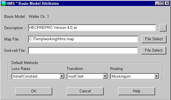
In this window, take a look at the Default Methods section. The
method on the left, Loss Rates, is where you choose the process
which calculates the rainfall losses absorbed by the ground. Click on ![]() in the Loss Rate section to see your choices. Some options are SCS
Curve No. and Green & Ampt. In this model, Initial/Constant
has been selected. This loss relationship means that a quantity of rainfall
will be absorbed by permeable soil initially, and a constant rate will
be absorbed over the time frame of the model.
in the Loss Rate section to see your choices. Some options are SCS
Curve No. and Green & Ampt. In this model, Initial/Constant
has been selected. This loss relationship means that a quantity of rainfall
will be absorbed by permeable soil initially, and a constant rate will
be absorbed over the time frame of the model.
The middle section, Transform, allows you to specify how to convert
excess rainfall to direct runoff. Again, click the ![]() to view your options, most of which you should recognize. This model employs
the SCS technique. The modClark model referred to above takes gridded
rainfall data, subtracts the losses as specified through the Loss Rates,
and converts the excess rainfall to a runoff hydrograph using a variation
of what is known as the Clark unit hydrograph. You may go
elsewhere to learn more about how the modClark method works.
In addition, Seann Reed, a graduate student working with Dr. Maidment,
performed some of the pioneering work on converting gridded rainfall to
runoff that the HEC used when writing the HMS. You may more read about
this in an
on-line copy of his Master's Report.
to view your options, most of which you should recognize. This model employs
the SCS technique. The modClark model referred to above takes gridded
rainfall data, subtracts the losses as specified through the Loss Rates,
and converts the excess rainfall to a runoff hydrograph using a variation
of what is known as the Clark unit hydrograph. You may go
elsewhere to learn more about how the modClark method works.
In addition, Seann Reed, a graduate student working with Dr. Maidment,
performed some of the pioneering work on converting gridded rainfall to
runoff that the HEC used when writing the HMS. You may more read about
this in an
on-line copy of his Master's Report.
The final part of the Default Methods considers Routing,
which is where you specify the process for routing a hydrograph through
a river reach. Once again, click the ![]() and look over the choices. The Muskingum is specified here, which
is the routing technique used for the reaches in this model.
and look over the choices. The Muskingum is specified here, which
is the routing technique used for the reaches in this model.
At this point, close the Basin Model Attributes window by clicking on Cancel at the bottom of the window. Now that we have considered the various loss, transform, and routing techniques to use, we will look at the actual parameters associated with the chosen techniques. Choose Data-Eds. on the Schematic window menu bar. Your choices should be
Select Loss Rate and then Initial/Constant first. The following window should appear.
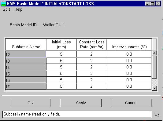
Note that while the Initial/Constant Loss Rate method was specified via another menu, it is in this table that the method parameters are actually entered. Each basin requires an initial loss quantity, a constant loss rate, and a percent imperviousness. These values have been selected arbitrarily. If the % impervious value differs from 0, that % of the land area is assumed to have no losses and the loss method is applied only to the remainder of the drainage area. Students in the Dept of Geography of the University of Texas at Austin, have studied how the growth of the University has changed the land use patterns over time in Waller Creek. See: http://www.utexas.edu/depts/grg/ustudent/gcraft/waller/waller.html
After you have looked over the data, click OK. For future reference, while both OK and Apply transfer the data to the computer's short-term memory, they differ only in that OK closes the window while Apply keeps the window open.
Once you have closed the Initial/Constant Loss window, choose Data-Eds., Transform, and then SCS to view this image:
![]()
Note that the SCS unit hydrograph method requires only one parameter for each sub-basin--lag time between rainfall and runoff in the subbasin. HMS. At this point, go ahead and close this window.
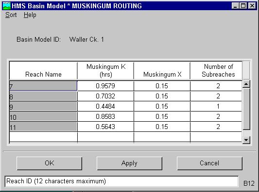
The next step involves entering the parameters for the routing process.
From Data-Eds., select Reach Routing and then Muskingum.
This should cause the following image to appear. This simulation
routes the water through the reaches by the Muskingum method in which K
is the travel time of a flood wave passing through the reach, X is a measure
of the degree of storage (X = 0 means a level-pool reservoir or maximum
storage, X = 0.5 means a pure transmission reach in which there are no
storage effects, and X ranges between 0 and 0.5). The reach is divided
into a number of subreaches if necessary to keep the computations numerically
stable.
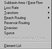
You do not have to go through the Data-Eds. menu to edit element properties. Editing may also be accomplished by highlighting an element, holding down the right mouse button, and choosing Edit from the pop-up menu. Before we move ahead to the precipitation data, close the Lag window and open Subbasin Area/Base Flow from Data-Eds., which should look like this:
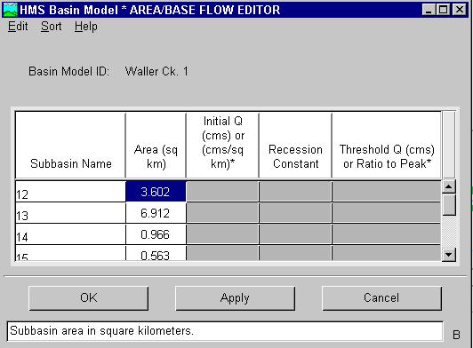
In this part of the HMS, you supply if necessary, information such as basin areas and initial base flows in the system. The recession ratio and threshold Q/ratio to peak values are used by the HMS to add baseflow to direct runoff. In this model we are not allowing for any base flow. When you are finishing with this window, close it. In addition, you should also close the Schematic window by selecting Close from the File menu.
To be turned in: Choose one of the subwatersheds and one of the river reaches and describe in words what the parameter values are that are used to characterize these features hydrologically.
3. Creating a Precipitation Model
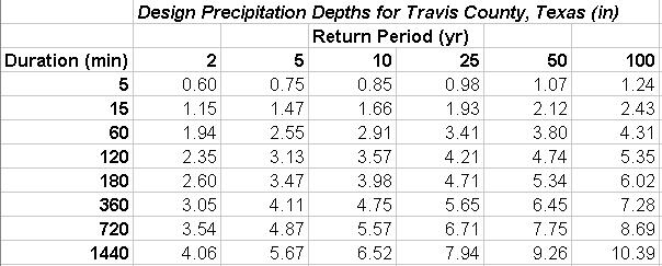
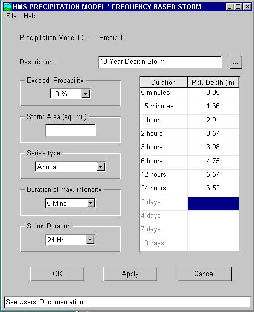
Having established the physical aspects of the model, we will now address the rainfall data. From a statistical study of extreme storm rainfall data recorded at gages, tables and maps have been prepared for the whole US which specify the storm precipitation depth to be expected as a function of the return period of the event and the duration of the rainfall. A table of such values is shown below for Travis County, in which the City of Austin is located. For example, for a 10 year return period event, we expect that in 5 min 0.85" of rainfall will fall, in 15 min 1.66", and so on, up to 720 min (12 hours) and 1440 min (24 hours). These precipitation depths are the values which would be equalled or exceeded on average once in 10 years when considering a very long period of data. The values shown for Travis County were extracted from a live map server accessible on the CRWR home page http://www.crwr.utexas.edu/texas/rainfall/. The values given in this server are precipitation intensities in mm/hr, so they were converted to depths in inches by multiplying by the rainfall duration and converting the resulting depth from mm to inches. As rainfall duration increases, the cumulative depth of rainfall increases but the average intensity over the duration decreases because severe rainfall cannot be sustained for very long.
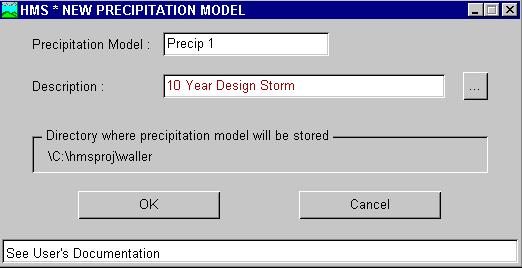
At present, HMS can handle rainfall input only in English units (inches). To create a design precipitation input file, go to the Project Window and select Edit/Precipitation Model/New. A window like this appears in which you can describe the precipitation file you intend to create, in this case for a 10 year storm.
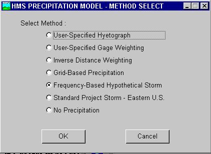
After clicking, OK, the following window appears, in which you should select the Frequency-Based Hypothetical Storm, as shown. The other options refer to different methods of inputting the precipitation data, including Grid-based Precipitation which comes from Nexrad radar.
When you click on Ok, the following table appears. Fill in the values shown from the table above for a 10 year storm (10% chance of being equalled or exceeded in any year). Click Apply, and then Ok to complete this step.
For each project, the HMS then creates an output Data Storage System DSS file which stores calculated data from all runs for a given project so that results from a previous run can be directly compared to results from a more current run. The HMS stores data in the DSS file according to the information given in the Pathnames section. F: is left blank because the HMS will place the name of the run there.
To be turned in: a screen capture of the design precipitation
input file
After you click Ok, you'll get the window to specify the duration of the simulation in date and time, and also the time interval of the calculations (10 minutes). In this case, the duration is arbitrary, long enough to depict the runoff from a 1-day storm, but the 10 minute time interval is part of the Basin file model setup and should remain fixed for this Waller Creek model.
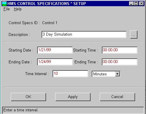
To be turned in: how many time intervals of computation will be performed?
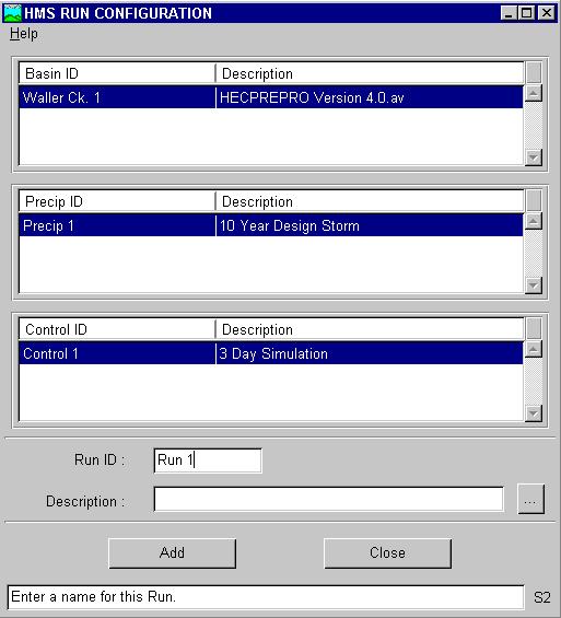
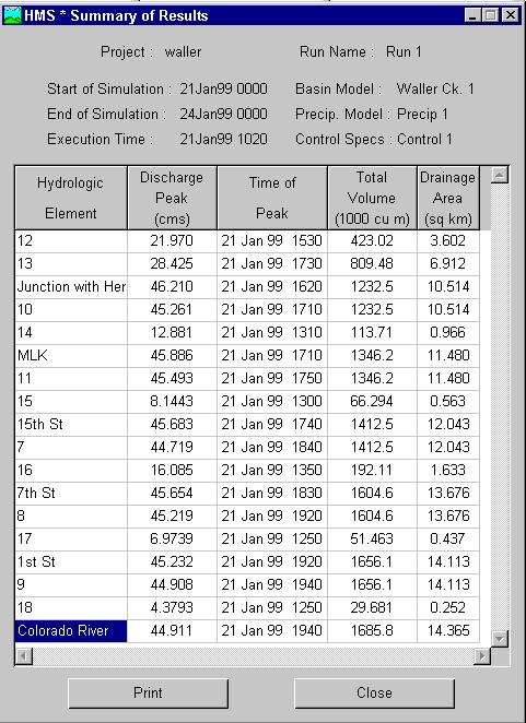
When finished, select Add, close the Run Configuration window, go back to the Project Definition, and choose Simulation Manager from the Simulate menu. You should see an image similar to this:
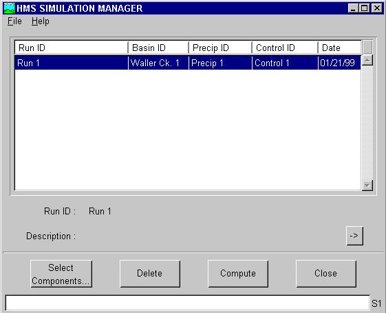
The Simulation Manager summarizes which Basin ID, Precip ID, and Control ID have been chosen for each run. In this window, Run 1 is composed of the three sets you just chose in the Run Configuration window. For the moment of truth, select Compute; if all goes well, you should see
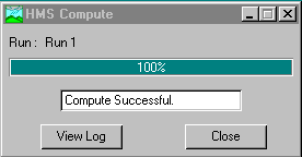
If you do not see this window, problems have arisen. If so, HMS gives a list of problem locations and by editing the Basin file you may be able to eliminate them.
In addition to viewing global results, you may also view results for
each element within the model. To do this, choose ![]() in the Schematic window, select an element in the model (Colorado
River for example) with the left mouse button, hold down the right mouse
button, and choose View Results from the pop-up menu which appears.
Pick from Graph, Summary Table, and Time-series Table.
If you view the Graph for Colorado River, you should see the following:
in the Schematic window, select an element in the model (Colorado
River for example) with the left mouse button, hold down the right mouse
button, and choose View Results from the pop-up menu which appears.
Pick from Graph, Summary Table, and Time-series Table.
If you view the Graph for Colorado River, you should see the following:
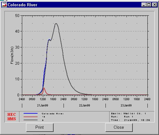
The light red hydrograph is the inflow data from the small area of Waller Creek immediately upsterm of the Colorado River which is added to the routed flow in the channel to produce the total outflow curve. If you click on a watershed, you see the rainfall at the top and the runoff at the bottom:

To be turned in: Make a table showing the peak discharge in cms at each of the six outlet points on Waller Creek (5 junctions and 1 sink).. What is the drainage area above each of these points? What is the peak discharge per unit of drainage area (cms/sq. km) for these points?
Study the data you are provided and if possible, improve the estimates of % impervious cover on the watershed, and the initial and continuing losses. The design is to be based on the 100 year design precipitation, not the 10 year storm that you've used up to this point.
To be turned in: a short account of your design discharge study. What input data values did you use? What design discharge at 15th St did you obtain? Show a graph of the discharge hydrograph at 15th St. How can you check the result to see if it is reasonable?
Go to Dr Maidment's Home Page