Example Application

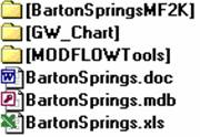
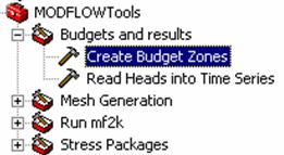
MODFLOWTools contains the installation package for installing the MODFLOW toolbox
Barton SpringsMF2K contains the modflow files used in the exercise
GW_Chart contains a charting tool to plot modflow results
Barton Springs.mdb is the geodatabase containing the GIS datasets
BartonSprings.xls contains discharge at three USGS gaging stations

Installing the MODFLOW tools:

If you have Windows XP you can use the installation wizard to install the tools. In the MODFLOWTools folder double click on the setup.exe file go through the installation wizard. The files will be installed under C:\Program Files\ModflowTools. It can occur that if you have an older version of Windows XP that the Setup file asks you to update your version of XP and then reboot the computer. If this happens, you need to register the tools manually.

Unzip the tools located in the zip file
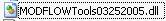
Locate the file MODFLOWTools03252005.dll in the MODFLOWTools folder and double click on the dll to register it.
Double click on the MODFLOWTools.reg file to register the toolbox.

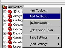
Once you have completed the installation you can open ArcMap and select to add a new toolbox by right clicking in the toolbox window.

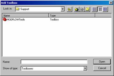
Browse to the Support folder in the MODFLOWTools folder and select the MODFLOWTools toolbox.

You are now ready to run the tools from ArcMap! Right click in the Arc Toolbox window and specify to save settings to default so that the toolbox always shows up when you open ArcMap.

Barton Springs segment of the Edwards aquifer:

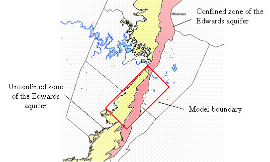
The Barton Springs segment of the Edwards Aquifer can be defined as the section of the aquifer that discharges to Barton Springs and Cold Springs. The hydrogeologic boundaries of this segment are a groundwater divide along Onion Creek in the south, and the Colorado River (Town Lake) in the north. To the west the aquifer is bounded by the Mount Bonnell fault and to the east the boundary is defined as the bad water line (where TDS exceeds 1,000 mg/l). A groundwater model was developed as part of the Texas Water Development Board groundwater availability models. The objective of the study was to evaluate long term groundwater availability in response to future pumpage and draught conditions (you can get the original model and model reports from the TWDB website at: http://www.twdb.state.tx.us/gam/ebfz_n/ebfz_n.htm).

Boundary of the MODFLOW model

The model grid consists of one layer constructed of 120 rows by 120 columns; each cell in the grid is 1000 ft long and 500 feet wide. Two models were developed; a steady state model for 1979 through 1998 based on average recharge during this time period and pumpage during 1989, and a transient model for a 10 year period (1979 through 1989) that includes periods of low and high water levels. Hydraulic conductivity was estimated by calibrating the model to the flow at Barton springs and to water elevations in monitoring wells. Throughout the exercise we will use a modified version of the steady state model to which transient stress periods were added.

Creating a GIS representation of the model

In this section of the exercise you will create a GIS representation of the MODFLOW model. We will focus on creating the model cells and nodes.

Creating MODFLOW cells and nodes

Open a new map in ArcMap document and save it.
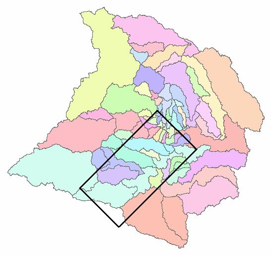
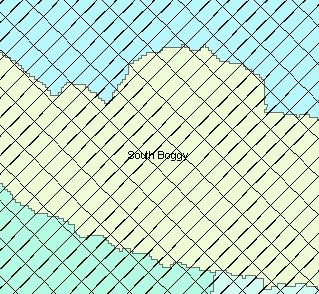
Load the Boundary, Watershed feature classes from the BartonSprings.mdb geodatabase. Symbolize the Watershed feature class using the Wshed attribute. You can see that the Boundary of the groundwater model that we will construct covers a number of watersheds.

Load the Nodes, Cell2D, and Cell3D feature classes from the BartonSprings.mdb geodatabase. These are empty feature classes that we are going to fill with Modflow model features.

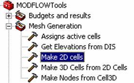
In the MODFLOW toolbox select the Make 2D Cells tool in the mesh generation toolset

· Browse to the Boundary feature class as the input boundary layer, specify the grid origin as upper left, the number of rows and columns as 120, the width as 1000 and the length as 500. For the output feature class browse to the Cell2D feature class in the BartonSprings feature dataset.

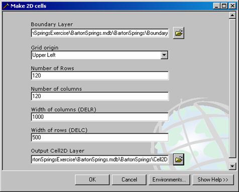
Select OK to run the tool

Once the tool is done you should see a set of polygons which represent the MODFLOW mesh cells. You can zoom in and use the identify tool to view the properties of the cells.

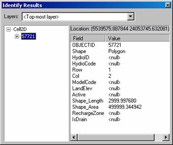
You can see that the area of the cell is about 500,000 square ft and that each cell has attributes describing the row and column of the model (in the above example Row = 1 Column = 2). All the MODFLOW inputs and outputs are based on the Layer, Row, and Column numbering system.

Within a model not all the cells need to be activated and only a portion of the cells are actually participating in the model calculations. Next you will define the active cells of the model.

Select the Assign active cells tool

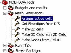
For the tools inputs select the Cell2D feature class, Active as the active field, Browse to the modflow files and select the BARTONMF2K.ba6 file as the input BA6 file and enter 120 for the number of rows and columns.

Select OK to run the tool

You can now view the active cells of the model by changing the symbology. (The active cells are in purple in the below figure). Active = 1 are the active cells. Set the Outline Color to No Color to avoid having the picture overwhelmed with black lines.

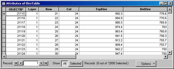
Model cells actually have three dimension properties. Each cell in a modflow grid has a top and bottom elevation associated with it. The elevations are stored in the discretization file (.dis). Next you will read the top and bottom elevations for each cell from the model files and store the values in a table.

Select the Get Elevations from DIS file tool

Select the Cell2D feature class as the input feature class, the LandElev field as the top elevation field, Row as the row field and Col as the column fields. Browse to the BARTONMF2K.dis for the DIS file and to the ElevTable in the geodatabase as the elevation table input.

Select OK to run the tool

You can open the elevation table and see that the top and bottom elevations for each cell were populated

Next you will create three dimensional cells from the 2D mesh and the elevations in the elevation table.

Select the Make 3DCells from 2DCells tool

As inputs select the Cell2D and Cell3D feature classes, the elevation table (ElevTable), and specify 1 as the number of layers. Select OK to run the tool.

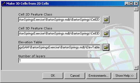
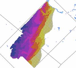
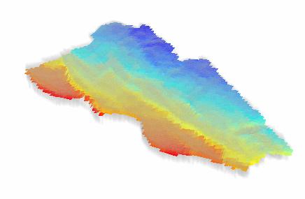
When the tool is done a set of 3DCells should be created. Each cell has a top and bottom elevation field and you can create a map showing the top or bottom elevations of the model. Below is a map showing the top elevations of the model.

Another way to view the cells is to use ArcScene to get a 3D view of the model mesh (To view the cells open ArcScene and load the 3DCells into the scene. You can change the vertical exaggeration under View > Scene Properties to get a better 3D view of the model).

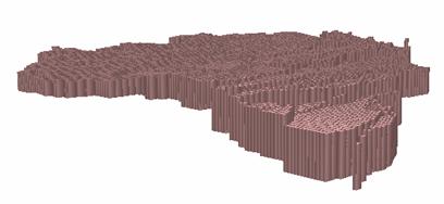
You can also load the DEM (demfeet) into the scene to show the model cells in comparison with the land surface.

To be turned in: What is the average thickness of the aquifer cells (ft)? What is the volume of solid materials encompassed by this aquifer (ft³)?

Next you will create the model nodes. MODFLOW is a finite difference model that uses a finite difference mesh to solve the groundwater flow equations. The model actually solves the head fields at the model nodes, which are located at the center of each cell.

Select the Make Nodes from Cell3D tool

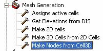
As inputs specify the Cell3D and Nodes feature classes. Select OK to run the tool

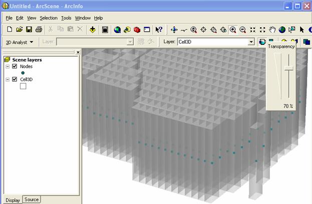
You can also view the nodes within ArcScene to see the three dimensional structure of the mesh.

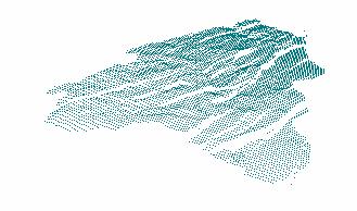
If you zoom in, and change the transparency of the Cell3D layer to 70%, you can see the nodes lie at the center of the cells.

If you zoom in you can see that there is a node at the center of each cell

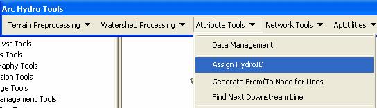
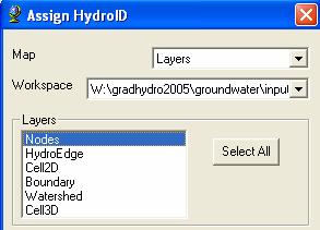
Later we will read model results (heads) based on the node feature class. We will use the ArcHydro time series structure, thus we need to assign HydroIDs to the nodes.

· In Arc Map Use the Assign HydroIDs tool in the Arc Hydro toolbar to assign HydroID values to all the nodes.

To be turned in: (1) A map showing the model boundary and model cells. Color the mesh by the active cell field to show the active part of the model. (2) A map showing the top elevations of the 3DCells.

Estimation of Groundwater recharge:

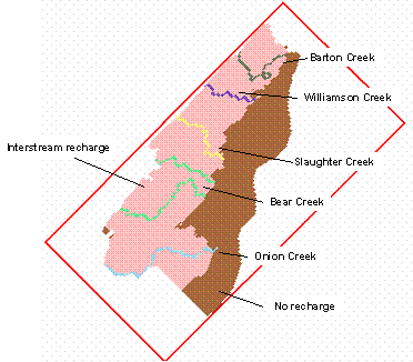
The primary source of recharge (about 85%) to the aquifer is from seepage from streams crossing the aquifer outcrop area. Flow losses from five major creeks (Barton, Williamson, Slaughter, Bear, and Onion) provide most of the recharge to this area. A linear relationship between streamflow at USGS gaging stations and recharge is used to estimate the recharge in all the creeks except for Barton Creek. Recharge increases linearly with flow in the upstream gaging station until a threshold of maximum recharge is exceeded and then the recharge is constant at that threshold. For Barton Creek, a cubic equation (Barrett and Charbeneau, 1996) is used to relate the flow in Barton Creek with recharge. In addition to recharge from the creeks diffuse interstream recharge is estimated at about 15% of the total recharge.

Recharge zones in the model

The main discharge sources are Barton and Cold springs, where Barton springs is the major discharge source accounting for 75 to 95 percent of the discharge.

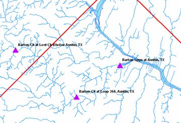
In the previous exercise you looked at stream discharge at two USGS gaging stations in Barton Creek (Lost Creek and station at loop 360). The hydrographs of measured upstream and downstream discharge indicated that the stream between the gages is a loosing stream. Groundwater recharge to the Edwards can be estimated based on measured streamflow at USGS gaging stations. The following set of equations describes the groundwater recharge from Barton Creek as a function of the flow at USGS gaging station 08155240 (Barton Creek at Lost Creek Blvd).

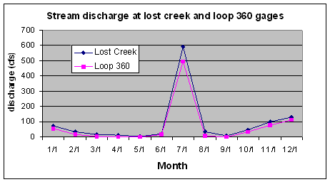
In the BartonSprings.xls spreadsheet you are provided with monthly mean streamflow measurements at Lost Creek Boulevard gaging station and at the downstream gage, Barton Creek at loop 360 (Gage number 08155300), for 2002. In addition you are provided with the discharge measurements at Barton Springs (Gage 08155500).

By plotting the streamflow discharge over time at the two gages you will see that the downstream gage has less flow than the upstream gage. This means that the stream connecting the two gages is a loosing stream (assuming there are no diversions between the two gages).

Recharge inputs to modflow

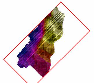
To translate the calculated recharge values into model inputs it is necessary to transform the recharge estimations from flows to fluxes. MODFLOW inputs require recharge values in the form of areal fluxes on cells in the modflow grid. In the Barton Springs GAM model Barton Creek is represented by a set of 50 cells (the green cells shown in the figure below)

Creating a potentiometric surface

In this section you will read model results to create a potentiometric surface within the aquifer. First we need to relate the model time domain to a date/time format. The modflow time discretization is based on stress periods. Each stress period has a length that defines the time interval in model units (in this model the units are days).

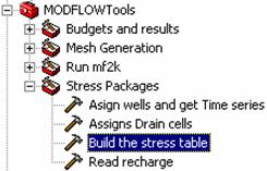
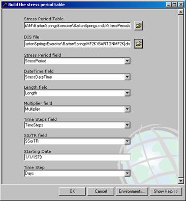
· Select the Build Stress table tool in the Stress Packages toolset.

· Select the StressPeriods table as the input table, BARTONMF2K.dis as the discretization file, specify the StressPeriod, StressDateTime, Multiplier, Length, TimeSteps, and SSorTR fields. The starting date of the model is 1/1/1979, and the time steps are Days. Select OK to run the tool.

After the model executes the stress periods table should be populated as shown below.

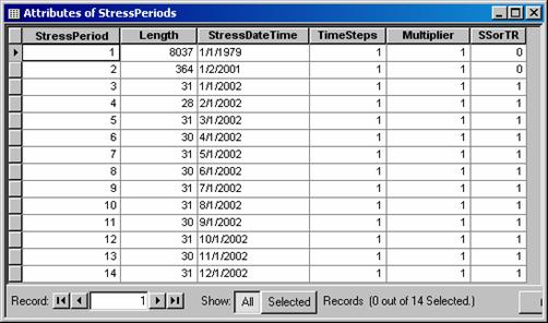
You can see that the model has 14 stress periods. The first two are steady state time steps (0 in the SSorTR field). The first two stress periods are from 1979 to 2000 and from 2000 to 2001. Then there are 12 transient stress periods, one for each month of 2002.

Next you will read in the heads simulated by the model.

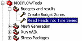
· Select the Read Heads into Time Series tool from the Budget and Results toolset

· Select the Node feature class and the TimeSeries table as the input files, specify BARTONMF2K.hed as the modflow head file, the starting date as 1/1/1979, TSTypeID as 1 , Time step as days, 1 layer, 120 rows and columns, and -9999 for HNOFLO (the value assigned to inactive cells). Select OK to run the tool.

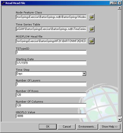
The tool reads the modeled heads from the modflow output head file and puts it into the ArcHydro time series format. Each node now has a set of time series in the TimeSeries table.

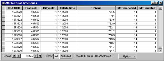
To create a potentiometric surface we need to extract information for one time step. As mentioned before two surfaces will be created one for January and one for July.

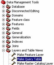
· In the general ArcToolbox, under Data Management tools select the Make Query Table tool

· Select the Nodes and the Time Series as the input tables, and select the select all fields option.

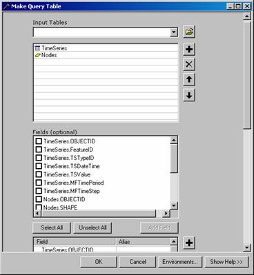
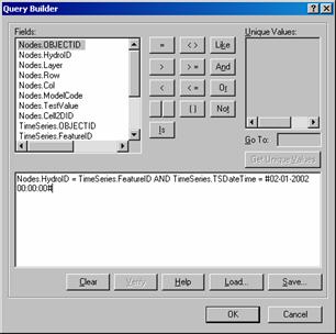
· Create a query in the Expression field to select only values for specific date (in the below example the date is 02/01/2002).

· Select the Add Virtual key field option. Select OK to run the tool.

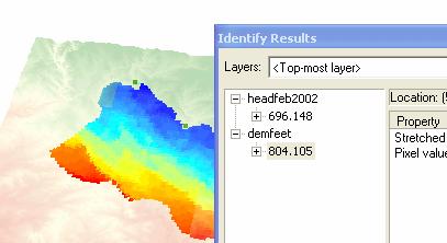
A new layer which joins the nodes with the time series should be created and added to the map. You can view the water elevations by symbolizing the layer based on the TimeSeries. TSValue attribute.

Next you will interpolate a surface from the nodes. Use the Spatial Analyst toolbar to interpolate a raster from the nodes with the time series.

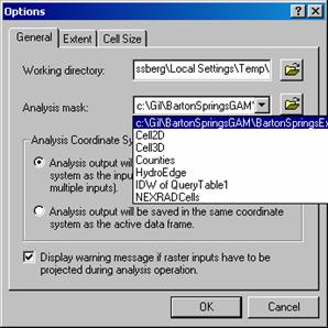
· Before running the interpolation, set the analysis mask in the spatial analyst toolbar. Go to Options > Analysis mask and select the Nodes feature class as the analysis mask.

· From the toolbar select the Interpolate to Raster tool, and select the (Inverse Distance Weighted) IDW method.

· Select the TimeSeries_TSValue attribute as the Z value field, 1200 as the output cell size, and leave all the parameters as the default parameters. Select OK to run the tool.

A raster representing the interpolated potentiometric surface should appear in the map.

Create contour lines showing the potentiometric surface within the aquifer to better visualize the surface.

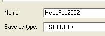
Make the piezometric head field a permanent grid

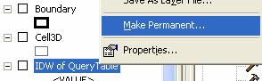
by saving as a grid HeadFeb2002.

In Arc Scene, add the HeatFeb2002 Grid and set the base height for display as follows:

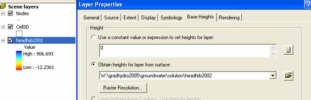
Add the Demfeet raster from the Rasters folder, set the layer height as above and visualize this in Arc Scene by varying the transparency of the layers

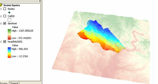
If you make the Cell3D transparent, you can see that the piezometric head surface lies within the elevation range of the cells. What does this tell you?

By moving the display you can see how much the piezometric head surface is below the land surface. By doing information queries at particular points you can see the discrepancy between these two elevations.

· Select the Contour tool in the Spatial Analyst toolbar

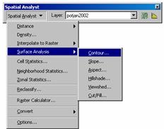
· Select 50 feet as the contour interval, and the base contour as 400.

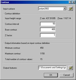
The contour of the potentiometric surface should be added to the map.

Load the EdwardsAquifer feature class, and symbolize the features based on the AQUIFER attribute. A value of 1 is for unconfined areas and values of 2 are for the confined zones.

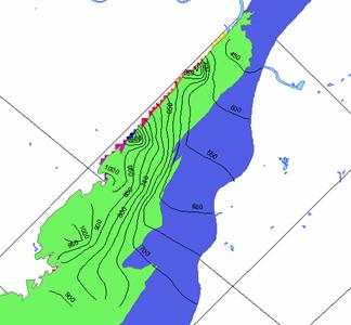
To be turned in (a) a map showing the contour lines of the potentiometric surface on top of the aquifer zones. Discuss the groundwater flow directions within the zones of the aquifer. (b) A 3D plot from ArcScene showing the DEM and piezometric head surfaces.

Creating water budgets:

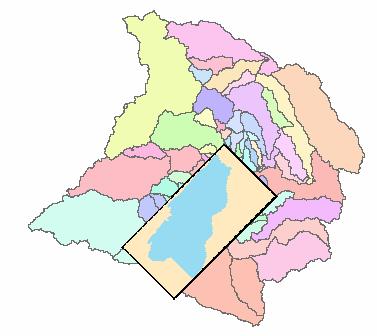
Zone Budget is an application that runs on top of modflow results files and creates water budgets for defined sub regions within the model. You will use a tool that runs zone budget to calculate a water budget for the Barton Creek watershed.

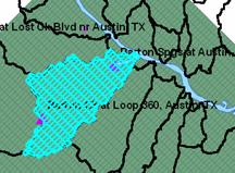
· Load the watershed feature class into the map, if it is not already there, and make the watersheds features hollow.

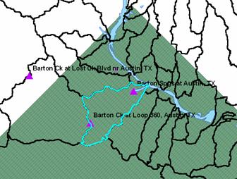
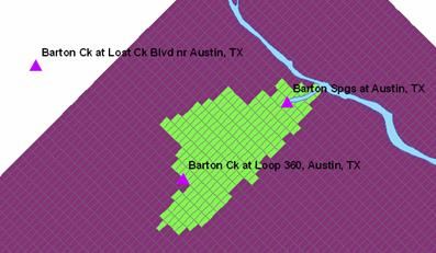
· Select the Barton Creek lower watershed (between Town Lake and the gaging station at loop 350).

Use the Select by Location tool to select all the 2DCells that are within the watershed

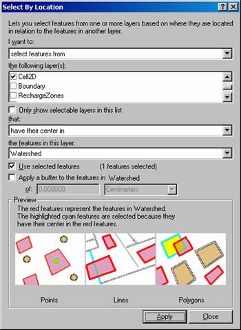
The cells within the selected watershed should be selected.

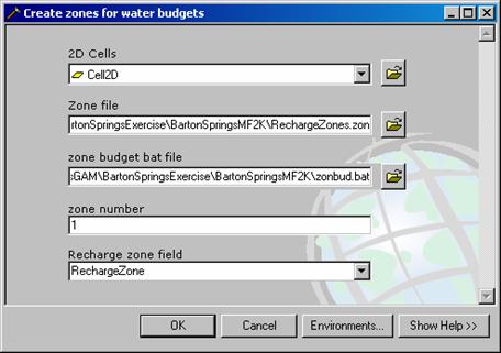
Select the create budget zones tool in the MODFLOW toolbox

Specify the Cell2D layer as the input layer, Browse to the file RechargeZones.zon (within the BartonSpringsMF2K folder) for the zone file, for the zone budget bat file select the file zonbud.bat, ()enter 1 as the zone number, and select the RechargeZone field as the recharge zone field. Select OK to run the tool.

Once the tool is done you should be able to show the defined zone by changing the Cell2D symbology based on the RechargeZone field.

The zone budget program creates an output file (bartonbudget.zbl) in the BartonSpringsMF2K folder that contains the water budget for the defined zone. You can view this data by opening the text file in NotePad.

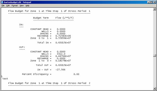
The above figure shows the zone budget for zone 1 (which you just defined) for stress period 1. The budget is in terms of total flow rate over the zone. In stress period 1 the recharge from the watershed to the aquifer is about 710,000 cubic feet /day, the flux from adjacent cells into the zone is about 5.6E+6 cubic feet /day. The selected zone also includes a cell representing Barton Springs, and the flux from the drain cell is about 4.47E+6 cubic feet /day. This means that the majority of the recharge fluxes from the watershed discharge at the springs.

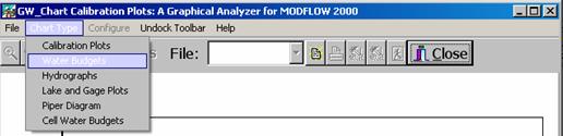
Another option for viewing the data is to use a charting tool developed by USGS for plotting modflow inputs and results. The name of the tool is GW_Chart and it is in the GW_Chart folder.

Click on the GW_chart.exe file to open the plotter
Select the water budgets option under the chart type

Select the open zonebudget file button (at the bottom right) to specify the budget input file. Select the bartonbudget.zbl file in the BartonSpringsMF2K folder.

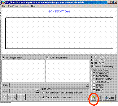
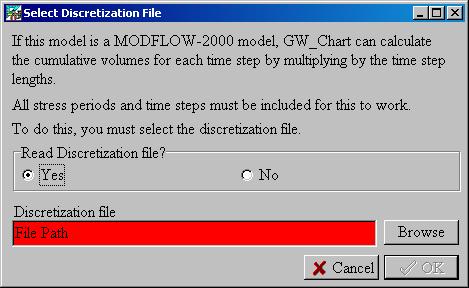
Select cancel when you are asked to select a discretization file.

The budget terms for the selected zone should appear on the plot. You can specify which terms you want to plot. Select to plot the in recharge as shown below.

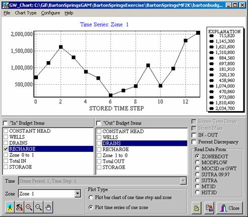
If you wish to extract data from the chart you can go into the Configure > Format Chart and select the Export and then the Data button. You should then be able to select the information you wish to copy from the chart.

To be turned in a plot of the recharge (In) and Drains (out) over time for the Barton Creek watershed between Town Lake and the gaging station at loop 360. The average discharge from Barton Springs is 53 cfs. How does the discharge from the drains compare to the average discharge?

Summary of items to be turned in:

1. What is the average thickness of the aquifer cells (ft)? What is the volume of solid materials encompassed by this aquifer (ft³)?

2. (a) A map showing the model boundary and model cells. Color the mesh by the active cell field to show the active part of the model. (b) A map showing the top elevations of the 3DCells.

3. (a) A map showing the contour lines of the potentiometric surface on top of the aquifer zones. Discuss the groundwater flow directions within the zones of the aquifer. (b) A 3D plot from ArcScene showing the DEM and piezometric head surfaces.

4. A plot of the recharge (In) and Drains (out) over time for the Barton Creek watershed between Town Lake and the gaging station at loop 360. The average discharge from Barton Springs is 53 cfs. How does the discharge from the drains compare to the average discharge?