Exercise 2. Water Balance of the
CE
394K.2
Spring 2005
Prepared by David R. Maidment and Jon Goodall
Table of Contents
Computer and data requirements
procedure
1. Viewing and querying the NARR files
2. Viewing and querying the ArcGIS RasterSeries data
3. Viewing and querying the ArcGIS Time series data
4. Constructing a water balance for 19-26
February
Summary of items to be turned in
The goals of this exercise are for you to become familiar
with the Arc Hydro TSWindow tools and to construct a
monthly energy balance and a daily water balance for watersheds in the
Computer and Data Requirements
This
exercise requires ArcGIS version 9.0 with the ArcInfo version
of the software operational and the Spatial
Analyst extension available, and also the Arc Hydro TSWindow,
an application package developed by Jon Goodall of
the Center for Research in Water Resources,
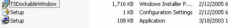
You can check whether the Arc Hydro TSWindow is already installed on the computer you are working on by using from the Windows menu Start/Settings/Control Panel/Add or Remove Programs. If the Arc Hydro TSWindow is installed, you’ll see it in the list as below.

In
the event that the ArcHydroTSWindow is not installed
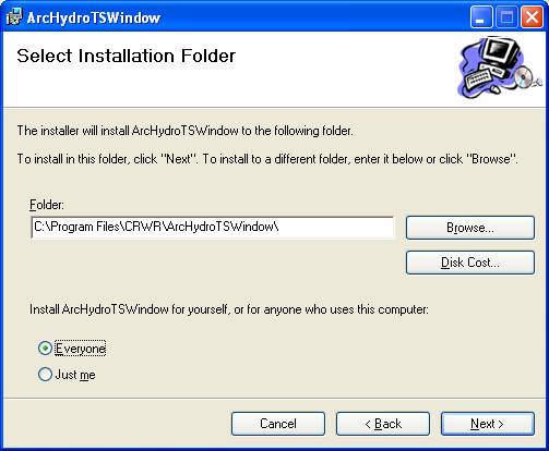
on the computer you are using, click on the Setup Application and you’ll be guided through by a Wizard through
the setup process. The second step in
that process gives you an option to install for yourself only or for everyone
who uses this computer, choose the Everyone option. Continue to the end of the installation. If you
have ArcMap open when you do the install, you’ll have
to close ArcMap and open it again in order for the TSWindow to operate correctly.
Data Files
The
data files are contained in a zip file ex2data.zip, which contains a geodatabase SanMarcosNARR.mdb,
and two folders SanMarcosNARR.idb
and 2003_NARRfiles, and a SanMarcosGeo
shape file that contains a map of the
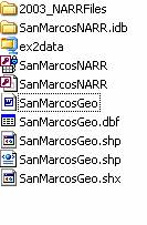
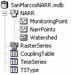
The SanMarcosNARR.mdb geodatabase contains a feature dataset NARR with three
feature classes:
MonitoringPoints
– stream gages in the San Marcos basin),
NARRPoints
– a set of points at the center of the NARR cells on a grid covering the San Marcos
basin)
Watershed – the 6 watersheds for the
San Marcos basin that we’ve worked with before)
RasterSeries
– a Raster Catalog that contains grids of NARR data interpolated from the NARRPoints)
Coupling Table – a table that links
features for each watershed needed to compute its water balance
TimeSeries
– an ArcHydro time series data table
TSType –
an ArcHydro time series typing table in a slightly
modified form
The SanMarcosNARR.idb
is a folder that contains a lot of .img files that
are actually the rasters referenced in the RasterSeries table shown the geodatabase.
The 2003_NARRFiles is a folder that contains files from the NARR-A for monthly energy balance over 2004, and for a daily energy and water balance during the week 19-26 February, 2003, which was a wet period in the San Marcos basin.
Download the Ex2data.zip file, copy it to a local directory and unzip its files.
1. Viewing and Querying the NARR files
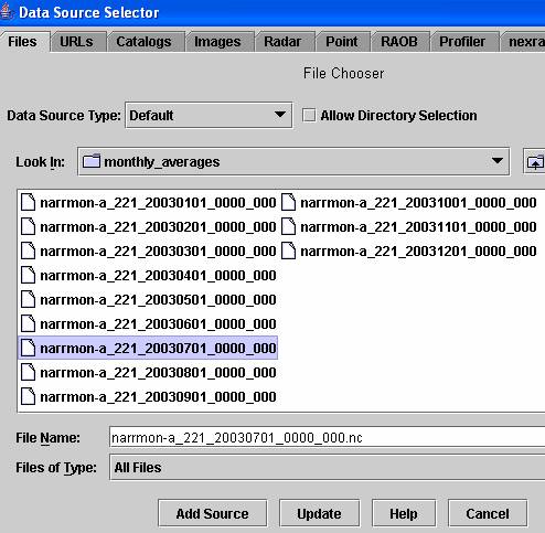
It is assumed at this point that you know how to use the Unidata Integrated Data Viewer. If not, please used Exercise 1, to learn how to do this: Ex1.htm Open the Integrated Data Viewer and use Data/New Data Source to navigate to the folder where you have stored the NARR files, go to the Monthly folder and used Add Source to open the file for July 2003:
![]()
Create a 2DGrid display of the Latent Heat
Flux at the surface of the earth. This
is the average latent heat flux in W/m2 for the month of July 2003, averaged over
all days of the month and over all hours of the day.
Use Displays/Map/Add
Your Own Map to add the map of the
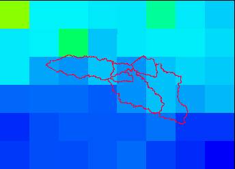
![]()
and here you’ll see our familiar
To
be turned in: For July 2003, what is the
range of variation of Latent Heat Flux for the region around the San Marcos
basin displayed in the NARR Grid? What
is the range of variation of the Latent Heat Flux within the basin?
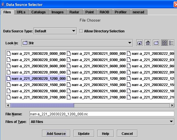
Add another Data Source by using Data/New
Data Sources, navigating to the 3Hr folder and selecting the folder for
1200z on
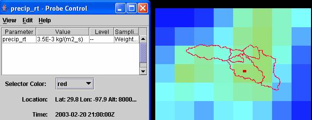
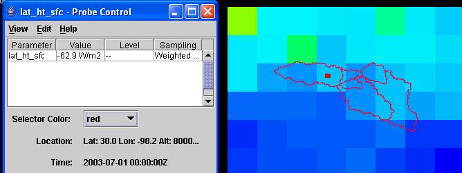
The data shown are the mass flux of
precipitation in kg/m2-s. You can convert this to
mm/hr by multiplying by 3600, thus 3.5 x 10-3 x 3600 = 12.6 mm/hr, and to in/hr
by dividing by 2.54, 12.6/25.4 = 0.50 in/hr – this is a fairly intense rainfall. Note that the time shown on the probe is
2100z and the time shown on the file is 1200z.
There is a discrepancy here, caused somewhere in the file conversions
necessary to acquire and pare down these data for local use.
To
be turned in: What is the range of
rainfall in inches/hour across the display at this time period?
2. Viewing and Querying
the ArcGIS Raster Series Data
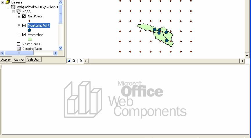
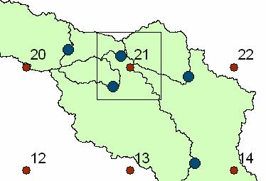
Open ArcMap and add the contents of the NARR geodatabase to the view
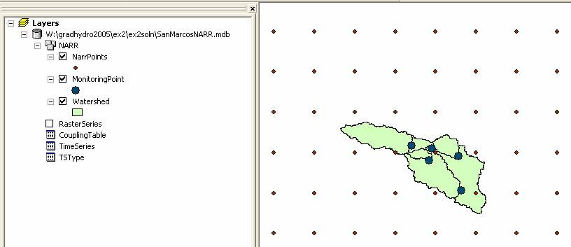
The
blue dots are streamgaging stations in the
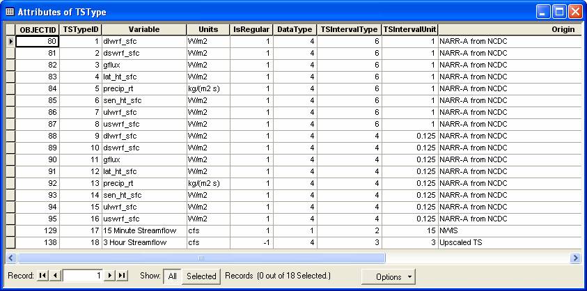
Open the TSType Table. You’ll see that you have 18 types of data stored in this display.
TSTypeID 1 – 8 are Monthly energy balance data from NARR (for the months of 2003)
TSTypeID 9 – 16 are 3 hour energy balance data from NARR (for 19-26 February 2003)
TSTypeID 17 is 15 minute streamflow from the NWIS (for 19-26 February 2003)
TSTypeID 18 is 3 hour streamflow data from NWIS (determined from the 15min data)
TSIntervalType = 1 second, 2 minute, 3 hour, 4 day, 5 week, 6 is month. TSInterval Unit is the number of TSIntervalType values the data interval is. Thus 0.125 of type 4 is 1/8 of a day or 3 hours, which is the same as 3 of TSIntervalType hours.
Lets check out the RasterSeries that we have for this basin. Open Arc Catalog and click on the RasterSeries folder. These rasters have been compiled by using Inverse Distance Weighting to construct a 1 km grid of data values for each variable and time interval of interest.
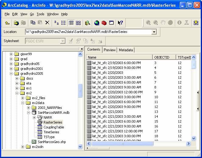
You see that you have rasters for TSTypeID 4, 5, 12, 13, in other words the latent heat flux (W/m2) and the precipitation rate (kg/m2-s) data for monthly intervals in 2003 and for 3 hour periods during the period 19-26 February, 2003. Both of these values are rates so the values given are average rates over the corresponding time interval. Scroll down in Arc Catalog to the Latent Heat Flux for June 30, 7PM (this is actually for July 1 at midnight in UTC time), the data for Arc Map have all been converted to Central Standard Time for this exercise. Click on this raster and drag it over onto the ArcMap display.
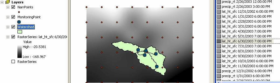
If
you click around using the Information tool ![]() in ArcMap you can
see the Latent Heat Flux in particular locations. Lets find the
average latent heat flux for the
in ArcMap you can
see the Latent Heat Flux in particular locations. Lets find the
average latent heat flux for the
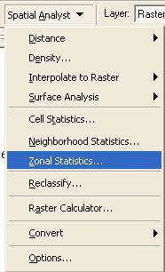
Set up the Zonal Stats tool table as shown below, making sure that you check the button to join the output table to the zone table:
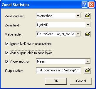
Click
OK to execute the Zonal Stats function.
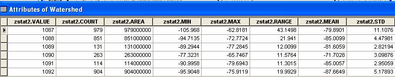
If you open up the Watershed attribute table now, you’ll see that you
have added data about average
latent heat flux to the Watershed feature class.
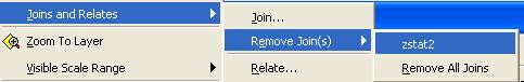
When you’ve completed compiling the values you need for this statistics query, right click on the Watershed feature class and eliminate the Join Table so you can repeat the exercise for the next time period or data set:
You can see from this exercise how much more powerful the spatial analysis functions are contained in ArcGIS compared to the query and display tools that you have with the IDV.
To be turned in: What is the average latent
heat flux for each of the 6 watersheds for July 2003 and for January 2003? What is the average latent heat flux for the
3. Viewing and Querying
the ArcGIS Time Series Data
We can also examine the NARR and flow data
using time series stored on spatial features like watersheds and stream
discharge gages. Open up the TimeSeries table and you’ll see lots of time series
information that is attached to the NARR points and the streamgage
points. The FeatureID
of the TimeSeries value is the HydroID
of the point to which it is attached.
There are 28,600 time series records shown, indexed by FeatureID and TSTypeID. They can thus be thought of as collections
of time series information of particular types attached to particular spatial
features.

In ArcMap, go to Tools/Customize

scroll down to TSWindow
and click on it. You should see a little
window pop up as shown below. If you
don’t have this option available to you in the tools menu, it means that you
haven’t installed the ArcHydro TSWindow. Go back to the beginning of the exercise, and
see the instructions about installing the TSWindow, close ArcMap and open it again,
and you should then have the display given below.
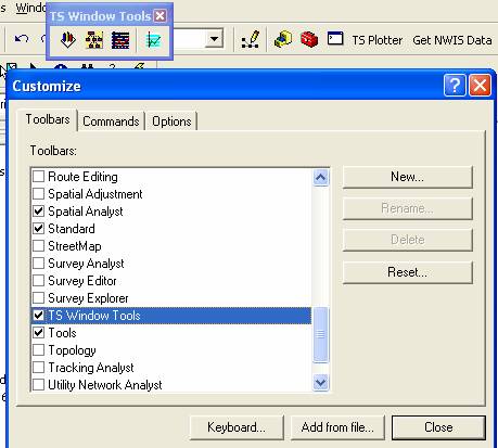
Hit Close to close the Customize Window.
The TSWindow has
four tools ![]()
![]() enables plots to be
made of Arc Hydro time series
enables plots to be
made of Arc Hydro time series
![]() allows a set of
graphical workspaces to be set up on which fluxes, flows and water balances can
be computed
allows a set of
graphical workspaces to be set up on which fluxes, flows and water balances can
be computed
![]() specifies where the
times series data are stored
specifies where the
times series data are stored
![]() creates a plotting
window in the ArcMap display.
creates a plotting
window in the ArcMap display.
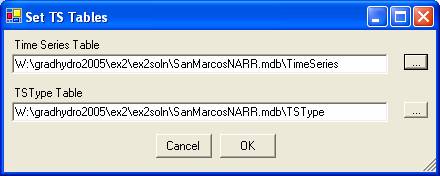
First, lets set the
time series locations. Click on the ![]() button and you’ll see the Set TS Tables
window. Navigate to where your time
series and TSType data are stored and click ok to set
the paths to those data. Save the ArcMap document so that you’ll have all this information
again if you need it.
button and you’ll see the Set TS Tables
window. Navigate to where your time
series and TSType data are stored and click ok to set
the paths to those data. Save the ArcMap document so that you’ll have all this information
again if you need it.
Now, lets open up a
graphing window. Click on the ![]() window and you’ll see a TS Chart window open.
window and you’ll see a TS Chart window open.

Drag this window down to the bottom of the ArcMap display and you’ll have a display window suitable
for plotting graphs.
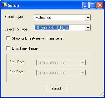
Click on the ![]() button and open the Setup window for plotting
time series. Select a Layer for which
you want to do plots, and automatically the data available for that layer are
available for selection in the box below.
button and open the Setup window for plotting
time series. Select a Layer for which
you want to do plots, and automatically the data available for that layer are
available for selection in the box below.

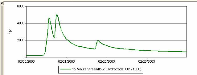
Click on any of the MonitoringPoint
features and the 15 minute flow data will plot.
Here are the 15 min flows for the
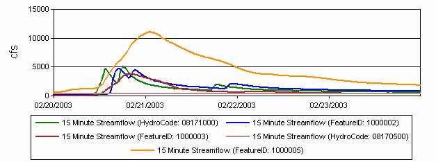
Here is a plot of all five streamflow records.
Where the HydroCode (USGS Site number in this
case) is populated in the TimeSeries table, that is
displayed, and where it is not populated the FeatureID
is shown as the data label.
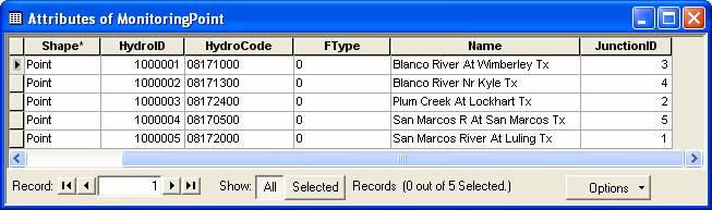
The values of these variables for the MonitoringPoint feature class are shown below:
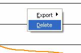
If you want to delete an existing chart,
right click in the chart display and select Delete:
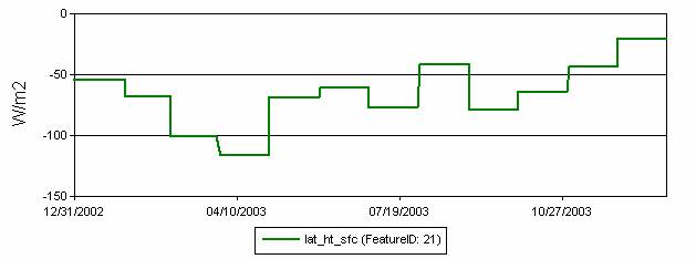
The Arc Hydro time series for the NARR points
can be plotted using:

which yields this plot for FeatureID
= 21 in the center of the
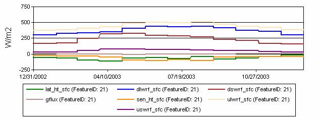
If you repeat this process from the beginning
(a bit tedious as the tool works now, but we’ll improve it later), you can plot
all the fluxes for FeatureID 21
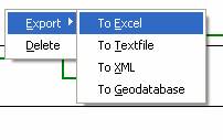
If you right click on a map display you can
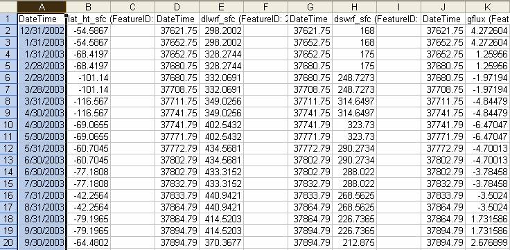
export the data to Excel
which produces a graph

and a worksheet with the data in it. The DateTime does not
write out in a convenient format but if you use Format Cell/Number/Date in Excel, you can get back a familiar date
format.
Arc Hydro time series have been compiled for
the Watershed feature class by automating the procedure that you just went
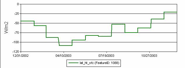
through to create a ZonalStats of the RasterSeries on the Watershed features. You can plot the monthly latent heat flux for
a watershed using
which yields for the watershed of the
To
be turned in: Construct a monthly energy
balance for each month of the year at the NARR point FeatureID
21. Does the energy balance close in each month? Make a plot that shows the
monthly variation of evaporation and precipitation for 2003 (each in mm/month)
for the Watershed of the
4. Constructing a Water
Balance for 19-26 February
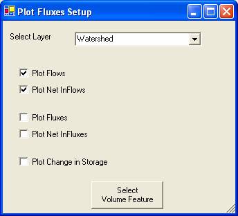
Hit the Plot Fluxes button ![]() and Select the Watershed feature class and the
options shown below. Hit Select Volume Feature.
and Select the Watershed feature class and the
options shown below. Hit Select Volume Feature.
As you move around the display you’ll see
features show up that measure fluxes or flows for a particular watershed. Here are the features for the
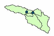
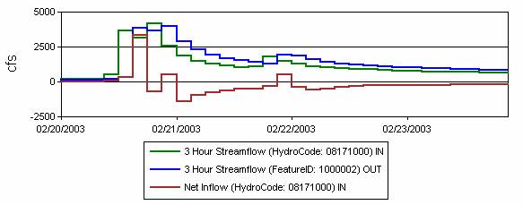
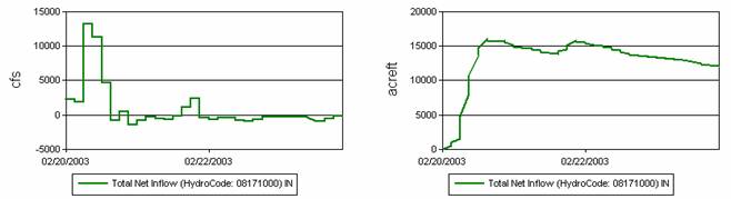
If you click on the watershed in between the
two gages shown you get a graph as below that gives the inflow, outflow and netinflow (inflow – outflow) for the stream gage flows.
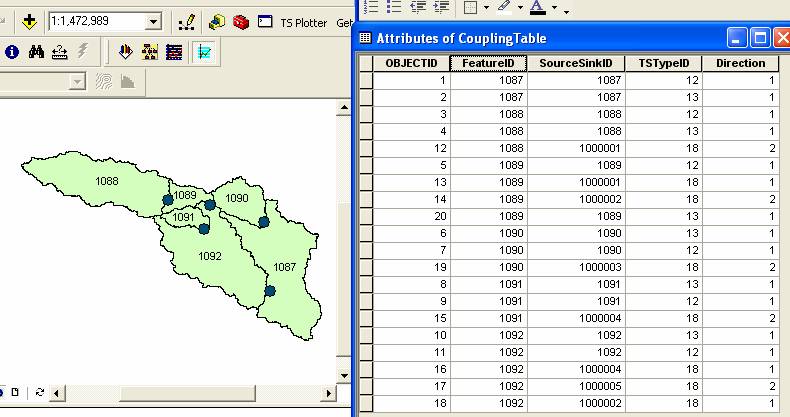
This is accomplished using a coupling table
as shown below that links features with the time series that describe them:
Similarly one can plot fluxes on this
watershed

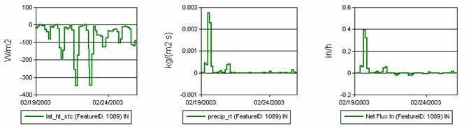
where the precipitation and evaporation data have
been automatically resolved to in/hr in computing the net flux.
You can drag graphs from one display to
another and they’ll show up in the new units.
There is lots more rainfall than evaporation in
this time period!
Finally, if you want to see all this put
together, plot change in storage

and if you right click on this graph, you can
accumulate the storage to give the storage through time on the watershed.

To
be turned in: Construct a 3 hour water
balance for Plum Creek at Lockhart and for the San Marcos River at San Marcos
for this time period. How do they
differ? Take the data for Plum Creek at
Lockhart into Excel and verify that the water balance computation is being done
correctly by reproducing the cumulative storage values.
Summary of Items to be turned in:
(1) For July 2003, what is the range of variation
of Latent Heat Flux for the region around the
(2) What is the range of rainfall in inches/hour
across the display at this time period?
(3) What
is the average latent heat flux for each of the 6 watersheds for July 2003 and
for January 2003? What is the average
latent heat flux for the
(4)
Construct a monthly energy balance for each month of the year at the NARR point
FeatureID 21. Does the energy balance close in each
month? Make a plot that shows the monthly variation of evaporation and
precipitation for 2003 (each in mm/month) for the Watershed of the
(5)
Construct a 3 hour water balance for Plum Creek at Lockhart and for the
OK, you’re done!