Exercise
1. Energy Balance of the San Marcos Basin
CE
394K.2
Spring 2005
Prepared by David R. Maidment and Jon Goodall
Table of Contents
Computer and data requirements
Procedure
1. Linking to the North American Regional Reanalysis
2. Select a data source
3. Prepare a
display
5. Map display of the San Marcos basin
6. Data Probe of the San Marcos basin
The goals of this exercise are for you to become familiar with the Integrated Data Viewer as a way of viewing and querying atmospheric science datasets for the energy balance of the earth, and to construct an energy balance for a typical day in July 2003 for North America, and for a location 29.9ºN and 97.9ºW in the San Marcos basin.
Computer and Data Requirements
Integrated Data Viewer
The
Integrated Data Viewer (IDV) is developed by Unidata, http://www.unidata.ucar.edu/ , a
program of the Universities Corporation for Atmospheric Research located in
Boulder, Colorado. With the sponsorship
of the National Science Foundation, Unidata supplies real-time feeds of
atmospheric science information for use in US academic institutions. IDV is a Java program that can be installed
in computers with a variety of operating systems. For use on machines with the Windows XP
operating system, the version InstallAnywhere
Windows installer for IDV (Direct3D) V1.1
(idv_1_1_windows_d3d_i586_installer.exe) is best. This can
be downloaded from http://my.unidata.ucar.edu/content/software/idv/index.html
once you have established a user name and password. To avoid having to do that, you can obtain
this version here: IDVinstaller This is a .exe file. Click on it to automatically install the
program. This installs the program
caller from your Start Menu, as shown below.
IDV is a public domain software program that is available free of
charge. It requires that Java already be
installed on the computer on which it will run.
For this exercise, we are going to use historical weather model data from the North American Regional Reanalysis (NARR), http://wwwt.emc.ncep.noaa.gov/mmb/rreanl/index.html which is an archive for 1979 to 2003 developed by running the Eta numerical weather prediction model of the National Centers for Environmental Prediction on an historical database of weather observations.
To be turned in: Make a brief summary of the North American
Regional Reanalysis – how was it produced, what data summaries does it contain,
what is its spatial extent and coverage in time?
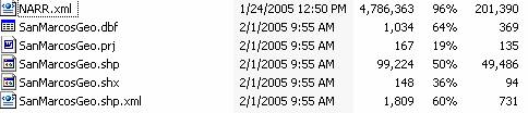
Data Files
The
data files for this exercise are available at ex1.zip
They consist of NARR.xml, an xml file that locates the North American Regional Reanalysis files,
and a shape file of the
1.
Making the link to the NARR
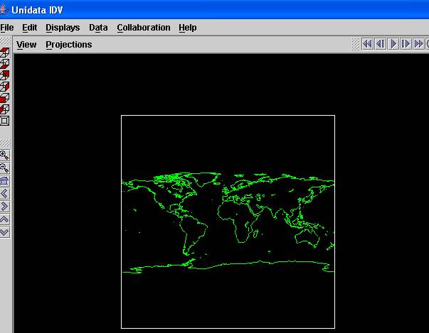
The IDV uses an XML file NARR.xml to locate the NARR data. You will actually be viewing the data while they remain resident in their remote location, not downloading them to a local file. Copy this NARR.xml file to your local directory. Open the IDV (use IDV not Globe IDV)
![]()
You’ll see a display like the one below with a map of the world.
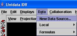
Select Data/New
Data Source, Make sure you are in
the Catalogs section of the Data
Selector window, not the Files section.
![]()
![]()
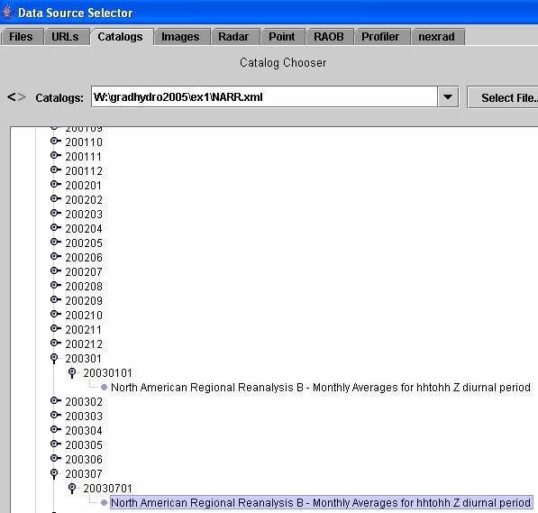
Hit Select File and then
navigate to the location of the NARR.xml file and select it. Hit Update
on the bottom of the Data Selector page to update the list of files available
at that location. You’ll get a display
that looks like this:
The NCEP HIRES GFSAVN and MESOETA are current
numerical weather prediction models whose data we are not going to use for the
moment. NARR-A describes the physical
condition of the atmosphere, while NARR-B stores the energy balance
components.
We will use the NARR-B_Monthly_3hr data.
Click on the radio button for this data set to expand it:
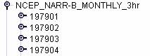
and scroll down to the January 2003 dataset,
and further expand it:

Click on the “North American Regional
Reanlysis B ….” to Add Source or add
it to the display as a new data source.
Expand the 2DGrid button see the fields available.
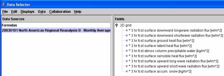
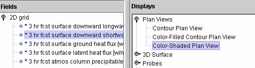
Select 3
hr fcst surface downward shortwave radiation flux [w/m^2] and select from the Display options Color-Shaded
Plan View.
and hit the ![]() button.
You’ll get a display like this:
button.
You’ll get a display like this:
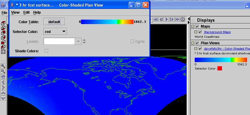
Click in the Color-Shaded Plan View window on the color ramp ![]()
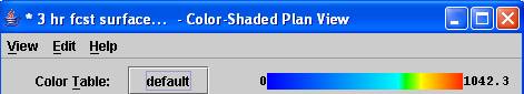
and from the options offered select Bright38
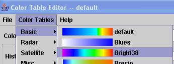
and hit
OK to apply it. Close the Color Shaded
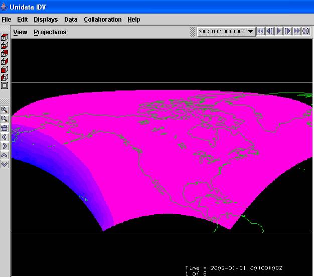
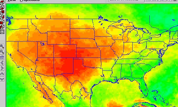
Plan View Window and you’ll see a display like this:
![]()
which shows that at
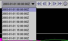
Select each one and view the progress of the
sun across North America during an average day in January 2003. What you are seeing is the esimated downwave
solar radiation for the given hour averaged across all the days of January
2003.
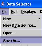
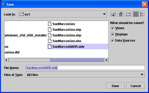
Its good at this point to save the display
you’ve created. To do this, using File/Save As from the main IDV Window
and save the file as
SanMarcosNARR.xidv. The extension .xidv
is a signal that this is an IDV map file.
Click on Data/New Data Source and select
NARR-B 3hr for July 2003:
Make a new display for this data source and
color it similarly to the January one (with Bright38). You’ll see that you can animate the two
images superimposed on top of one another using the animation toolbar ![]() . If you end up with repeated displays of the
same dataset, you can get rid of the unwanted ones with the little garbage can
on the right hand side of the legend display.
. If you end up with repeated displays of the
same dataset, you can get rid of the unwanted ones with the little garbage can
on the right hand side of the legend display.
![]()
To
be turned in: Make a display of the
downward solar radiation for each of the 3 hr intervals for January 2003 and
make a similar series of 8 maps for July 2003.
At what Z time does the maximum solar radiation occur? Where is the maximum solar radiation located
for January? Where is the maximum solar
radiation for July? The data you are
viewing are solar radiation at ground level, not at the top of the
atmosphere. Why is there more solar
radiation in the western US during July than in the eastern US?
5. Map Display of the
Now lets focus in on the
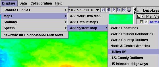
and you’ll get a display with the Hi-Res US
like below.
You can use the zoom and arrow tools on the
left side of the display to zoom in and center your picture. If the color of an added map is not what you
want, click on Map Display ![]() to bring up an editor that lets you change the
map colors.
to bring up an editor that lets you change the
map colors.
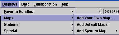
To add a map of the San Marcos basin, Add
Your Own Map,
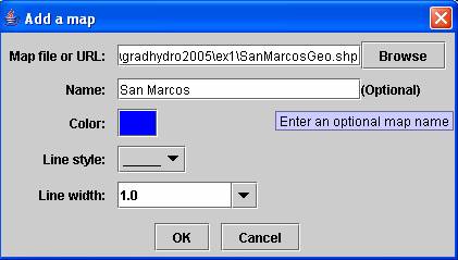
You’ll get a display that says “Add a Map”,
hit the Browse button
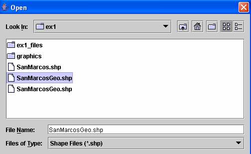
and you’ll get a new window that says Open, Select Files of Type Shape Files (*.shp) at the bottom of the page
and you can select individual shape files.
You can then rename the map to San
Marcos in the Add a Map window
above. There is a repeated image in the
picture below of SanMarcosGeo.shp because there is a SanMarcosGeo.shp.xml file
also in the list. Make sure you choose
the .shp file that does not have the .xml extension.
Note that maps must be in geographic coordinates to display correctly in the
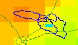
IDV. You can zoom in on a view of the
San Marcos basin with interstate highways also displayed to give a sense of
location (highways around Dallas-Fort Worth, Houston and San Antonio are shown
in this map). It seems that the IDV can
display line or area shape files but I am not sure if it can display point
shape files.

It’s a good idea to use File/Save As to resave your IDV map images now.
To
be turned in: A map display showing the San Marcos basin overlying a short wave
radiation flux map.
6. Data Probe of the
Now we are going to set up a Data Probe,
which is a query tool to get values from the display. As shown below, open up a new display of the
3 hr fcst surface downward radiation flux 2D Grid.

Now, instead of selecting a map display,
select the Data Probe
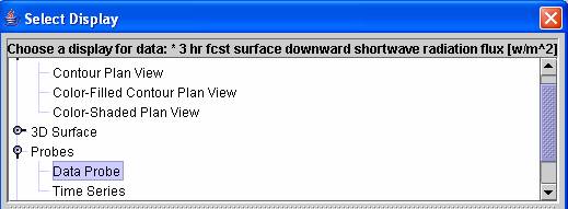
You’ll see a window that says Probe Control,
and a little blue box in the map display.
(you might have to zoom out to find the little blue box).

As you move the little blue box around,
you’ll see the values in the Probe Display change. Fix the probe location at 29.9°N and
97.9°W. This is just where the outlet of
the San Marcos River at San Marcos occurs by IH-35 (at the campus of Texas
State University).
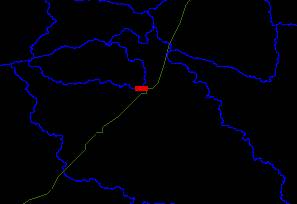
Cycle through the map displays and you’ll see
the values under the probe change:
If you right click in the Table of the Probe,
use the Edit option in the Probe
Table, you can add additional parameters
to be measured at the probe, and you can also delete parameters. It seems that the probe can handle up to 6
parameters in its display. Since our
problem has seven fields that we want to examine, you can do this in two passes,
adding or deleting fields from the probe table as required.

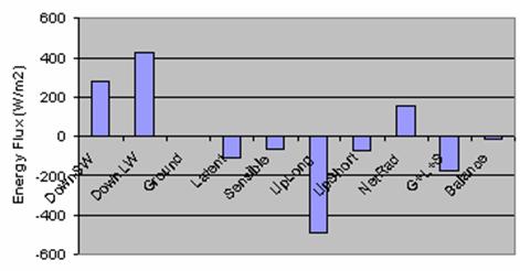
Here is a graph showing the various energy
balance components through the day for July, 2003.
Here is a plot of daily average values of the flux components. The upward longwave and shortwave components have been made negative in this plot to indicate that they are energy losses from the earth’s surface. Net radiation = DownSW + DownLW – UpLong – UpShort. This net radiation is consumed by ground heat flux (G), latent heat flux (L) and sensible heat flux (S). The balance is the sum of the net radiation and G + L + S. It should theoretically go to 0.
To
be turned in: Make a table showing the
Downward Short Wave Radiation values for 29.9°N and 97.9°W for each three hour
interval during the day in July. Make a
similar listing for the values of
1.
Downward Longwave Radiation Flux
2. Downward Shortwave Radiation Flux
3. Ground Heat Flux
4. Latent Heat Flux
5. Sensible Heat Flux
6. Upward Long Wave Radiation Flux
7. Upward Short Wave Radiation Flux
Make
graphs showing data series 1-7as a function of time of the day.
What
is average July evaporation in mm/day at this location?
Use
the NARR to make another energy balance study of your own devising. Compare the values you obtain for the period
you choose with the ones that you’ve obtained above for July 2003.
Ok, you’re done!