Flow Routing on Barton Creek using
HEC-RAS
Prepared by Venkatesh Merwade
CE 394 K.2 Surface Water Hydrology
Spring 2005
Introduction
The goals of this exercise are:
·
Give you an understanding of how the HEC-RAS
model is run for unsteady flow analysis on Barton Creek between
· Understand the hydrologic processes along the Barton Creek by comparing the outflow hydrograph from the model with the observed hydrograph.
The model’s geometry data and unsteady flow data are stored in BartonRAS.zip file at http://www.ce.utexas.edu/prof/maidment/gradhydro2005/Routing/BartonRAS.zip Download BartonRAS.zip and unzip it to a working directory (BartonRAS) on your computer.
BartonRAS.zip has the following files:
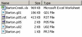
BartonCreek.xls:
MS Excel file that contains flow and stage data for the two USGS gaging
stations (Barton Ck at
Barton.g01: HEC-RAS Geometry File for Barton Creek. Geometry files contain all of the geometric data for the river system being analyzed. The geometric data consist of: cross section information; hydraulic structures data (e.g., bridges and culverts); coefficients; and modeling approach information. For this exercise, we are only using the channel geometry data and there are no structures/bridges in the geometry file (Geometry files have extension from g01 to g99. The "g" indicates a Geometry file, while the number corresponds to the order in which they were saved for that particular project.).
Barton.p05: HEC-RAS Plan File for Barton Creek. The plan file contains: a description and short identifier for the plan; a list of files that are associated with the plan (e.g., geometry file and steady/unsteady flow file); and a description of all the simulation options that were set for the plan. (Plan files have the extension .p01 to .p99. The "p" indicates a plan file, while the number represents the plan number).
Barton.u02: Unsteady Flow Data File for Barton
Creek. Unsteady flow data files contain: flow hydrographs at the upstream
boundaries; starting flow conditions; and downstream boundary conditions. (Unsteady
flow data files have the extension .u01 to .u99. The "u" indicates an
unsteady flow data file, while the number corresponds to the order in which
they were saved for that particular project)
Barton.prj: HEC-RAS Project File for Barton Creek (not a projection file for GIS!). The Project File contains: the title of the project; the units system of the project; a list of all the files that are associated with the project; and a list of default variables that can be set from the interface. Also included in the project file is a reference to the last plan that the user was working with. This information is updated every time the project is saved.
Starting a HEC-RAS project
To start HEC-RAS go to StartàProgramsàHECàHEC-RAS 3.1.1.. as shown below (HEC-RAS 3.1.1 is installed on computers in Civil Engineering Learning Resources Center):
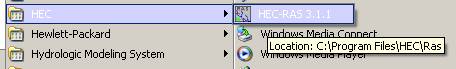
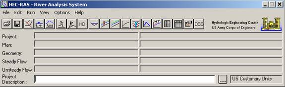
Click on HEC-RAS 3.1.1 to get the HEC-RAS interface as shown below:
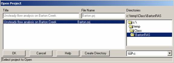
Click on the open project command button ![]() , browse
to your working directory, and highlight the project titled “Unsteady Flow Analysis on Barton Creek”,
file Barton.prj (shown below). Click
OK.
, browse
to your working directory, and highlight the project titled “Unsteady Flow Analysis on Barton Creek”,
file Barton.prj (shown below). Click
OK.
On the HEC-RAS interface, the project, plan, geometry and unsteady flow information should now be filled with the names of those respective files as shown below:

Note that the project now has a Plan file, Geometry file and Unsteady flow file in it. Lets examine the contents of geometry file and unsteady flow file.
Channel Geometry
The channel geometry (cross-sections) that is used in the
exercise is created by using River Channel Morphology Model (RCMM). RCMM uses
the shape of the channel in conjunction with flow data to describe the
three-dimensional structure of channel cross-sections. Select EditàGeometric
data…. or click on geometric editor button ![]() to see the plan view of the reach of the
Barton Creek between Lost Creek Blvd and loop 360 as shown below:
to see the plan view of the reach of the
Barton Creek between Lost Creek Blvd and loop 360 as shown below:
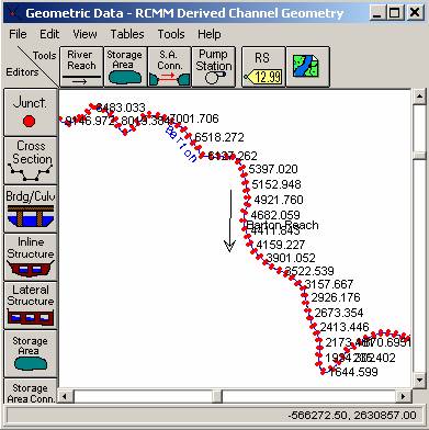
Select ViewàZoom In… to have a close look at the cross-sections as shown below:

What you see in the above figure is a plan view of a set of
cross-sections along the Barton Creek with labels measuring the river station,
or distance in meters from the downstream end of the creek. River stationing
for the reach under study starts at the downstream gaging station (Barton Creek
at loop 360) and continues up to the upstream end (Barton Creek at
In the plan view, each cross-section can be viewed in detail by selecting the “Edit and/or create cross-sections” button as shown below:
![]()
The figure below shows the cross-section with River Station = 9146.972 (this is the most upstream cross-section in the reach). In the table on the left (Cross Section X-Y Coordinates), Station (this station is different than River Station) refers to the distance from the left side of the cross-section (looking downstream), measured in feet, while elevation is the elevation above mean sea level in feet.
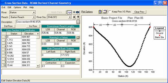
The Downstream Reach Lengths refer to the distance in meters to the next downstream cross-section (LOB is left over bank, Channel is the main channel and ROB is right over bank). Manning’s n Values are the n values for LOB, Channel and ROB, respectively. The Main Channel Bank Stations refer to the Station values of the two red dots in the plot, and the Contraction and Expansion Coefficients refer to the coefficients for the minor head losses associated with changes in channel cross-sections.
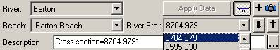
A different cross-section can be viewed by using the ![]() arrow keys or choosing a River Station from
the river station combo-box as shown below:
arrow keys or choosing a River Station from
the river station combo-box as shown below:
Similarly, reaches can be changed by using the corresponding
boxes. If a parameter is changed manually for any cross-section, the geometry
file can be updated by clicking the Apply Data button on the top. The
cross-section display on the right side can be turned on or off by using the
hide XS plot ![]() button.
button.
Close the Cross Section Data and Geometry Data windows to get back to the main River Analysis System window.
Unsteady Flow Data
The flow data for this exercise are extracted from USGS and are stored in BartonCreek.xls. The stage and flow data available from USGS are in US Customary Units. Now lets look at the unsteady flow data. From the main menu, select EditàUnsteady Flow Data… to open the unsteady flow data editor as shown below:
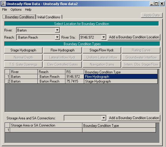
The purpose of unsteady flow data editor is to input initial and boundary conditions for simulating unsteady flow in the channel. Click on Boundary Conditions tab to look at the boundary conditions for the model. There are 12 types of boundary conditions that can be specified for unsteady flow simulation. However, not all 12 types apply to a single boundary condition location, and only one type of condition can be chosen for any single location. For example, in the above figure, three types of boundary conditions apply for an upstream boundary condition location (Stage Hydrograph, Flow Hydrograph and Stage/Flow Hydrograph). Flow Hydrograph is the most commonly used upstream boundary condition. If you click on the downstream boundary condition, you will notice that two more boundary condition types (Rating curve and Normal Depth) become active as shown below:
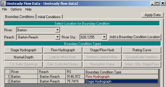
We will use the Stage Hydrograph boundary condition for this exercise. The boundary conditions data are already entered for this exercise. If you had to add a new boundary condition location, this could be done by choosing the Reach and River Station, and then clicking the Add a Boundary Condition Location button. The boundary condition is then entered by clicking on the appropriate Boundary Condition Types button. Double click on the boundary condition type (Flow Hydrograph) for the most upstream cross-section (RS = 9146.972) to see the inflow hydrograph as shown below:

The inflow hydrograph is entered manually by using HECRAS input sheet in BartonCreek.xls. You can also plot the hydrograph by using the Plot Data button as shown below:

Close the Flow Hydrograph and the boundary condition window to go back to unsteady flow editor. Double click on the downstream boundary condition type (Stage Hydrograph) for the most downstream cross-section (RS = 75.7415) to see the inflow hydrograph as shown below:

The stage hydrograph is entered manually by using HECRAS input sheet in BartonCreek.xls. You can plot the stage hydrograph by using the Plot Data button on the bottom. Close the stage hydrograph window.
In the unsteady flow editor window, select the Initial Conditions tab to provide initial conditions for the model. As shown in the figure below, there are two options for providing initial conditions. The first option is to enter flow data for the reach (typically the first ordinate of the inflow hydrograph) and have the program perform a steady flow run to compute the corresponding stages at each cross section. This is the most common method for establishing initial conditions.
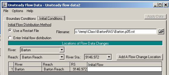
The second option is to read in a file of stages and flows that were written from a previous run, which is called a “Restart File”. We will use a restart file Barton.p05.rst in this exercise. Sometimes the program becomes unstable with bad initial conditions, so it is a good idea to use a restart file. HECRAS creates a restart file after each run. Save the unsteady flow data and exit the unsteady flow data editor.
Unsteady Flow Simulation
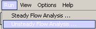
We are now ready for unsteady flow simulation. From the Run menu, select Unsteady Flow Analysis… as shown below:
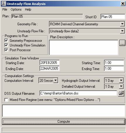
In the unsteady flow analysis window, check Geometry Preprocessor, Unsteady Flow Simulation and Post Processor. Each of these options is briefly described below:
Geometric Pre-Processor: The pre-processor is used to process the geometric data into a series of hydraulic properties tables, rating curves, and family of rating curves. This is done in order to speed up the unsteady flow calculations. Instead of calculating hydraulic variables for each cross-section during each iteration, the program interpolates the hydraulic variables from the tables. The preprocessor must be executed at least once, but then only needs to be re-executed if something in the geometric data has changed.
Unsteady Flow Simulation: The unsteady flow computations within HEC-RAS are performed by a modified version of the UNET (Unsteady NETwork model) program. The unsteady flow simulation is actually a three-step process. First a program called RDSS (Read DSS data) runs. This software reads, and converts all of the boundary condition time series data into the user specified computation interval. Next, the UNET program runs. This software reads the hydraulic properties tables computed by the preprocessor, as well as the boundary conditions and flow data from the interface and the RDSS program. The program then performs the unsteady flow calculations. The final step is a program called TABLE. This software takes the results from the UNET unsteady flow run and writes them to a HEC-DSS file.
Post-Processor: The Post Processor is used to compute detailed hydraulic information for a set of user specified time lines during the unsteady flow simulation period. In general, the unsteady flow computations only compute stage and flow at all of the computation nodes, as well as stage and flow hydrographs at user specified locations. If the Post Processor is not run, then the user will only be able to view the stage and flow hydrographs and no other output from HEC-RAS.
Specify the Starting and Ending date as
You will see the computing progress as shown below:
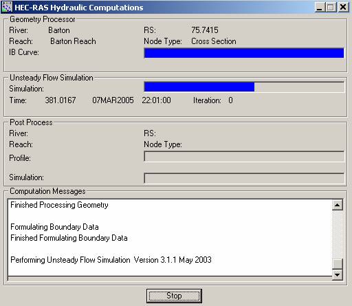
If you see too many messages in the computation messages window, the program has probably gone unstable!
For this exercise, there is some problem with the post-processing, and the following error message is displayed:
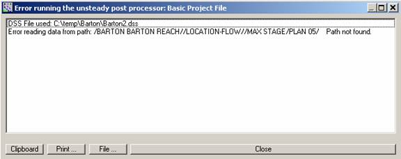
Post-processing is important for visualizing the results in HEC-RAS, but is not a very critical component for this exercise. We are interested in knowing the outflow hydrograph at the downstream cross-section as a function of inflow hydrograph at the upstream cross-section. This hydrograph is already computed before post-processing. Post-processor uses the results from unsteady flow simulation to calculate several hydraulic variables at each cross-section, which we do not need in this exercise. Close the error message box.
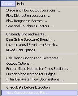
Now we will extract the results from unsteady flow simulation, which are stored in an ASCII file with *.bco extension. In the unsteady flow analysis window, select OptionsàView Computation Log File… as shown below:
This will open a text file (which will take a while to open). Scroll all the way down to see the outflow hydrograph at Station = 75.7415 as shown below (you can look at other things in the file to see what happened during the unsteady flow computation):
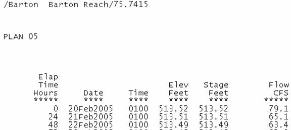
Copy the out flow hydrograph, save it in a separate text file (Barton_hyd.txt), and open this text file in an excel sheet to plot the outflow hydrograph. Save the excel sheet as Barton_results.xls. Also plot the inflow hydrograph at the upstream station and the observed hydrograph at the downstream station on the same graph. These can be copied from Daily Flow and Stage Data sheet in BartonCreek.xls. The final plot is shown below:
The segment of Barton Creek that we modeled in this exercise lies above the Barton Springs segment of Edwards aquifer. Also, we did not include the flows from tributaries while routing the inflow hydrograph. Keeping these two things in mind, answer the following questions and turn-in your homework!
To be turned in:
- A table and a graph with date, observed inflow hydrograph, observed hydrograph and model hydrograph? In the table, include an extra column to show the difference (+/-) between the observed outflow hydrograph and model hydrograph.
- A plot showing a close-up of the peaks between observed inflow hydrograph and observed outflow hydrograph (you can use the hourly data for March 6th and March 7th given in 15 Min Flow and Stage data sheet in BartonCreek.xls to prepare this plot)
- How
long does it take for the peak flow to travel the flow from Barton Creek
at
- Write a paragraph answering the following questions:
After you look at the two plots prepared in questions 1 and 2, what do you thinks is going on? Why is the model outflow hydrograph does not match with the observed outflow hydrograph? Why is the peak of the observed outflow hydrograph is higher than the inflow hydrograph? Why is the flow at the downstream end is lower than inflow hydrograph during low flows?