Eric Tate
CE 394K.3
May 7, 1998
etate@eqe.com
GIS Term Project
Display of Flood Levels in a GIS
Table of Contents:
- Introduction
- Run HEC-RAS
- Extract the RAS Stream Information
- Choose the Digital Stream
- Establish the Stream Boundaries
- Add the Cross-Sections
- Future Work
- Data Dictionary
In recent years, there have been numerous technological advances in the field of
geographic information systems (GIS). A recent thrust in GIS development has been
the use of GIS in conjunction with existing computer models. For my GIS term
project, I have attempted to link GIS to a hydraulic river model called HEC-RAS.
Since the mid 1960's, the standard computer program for modeling river and floodplain
hydraulics has been HEC-2, designed by the Hydrologic Engineering Center (HEC)
of the U.S. Army Corps of Engineers. In the early 1990s, HEC released the Windows
version of HEC-2, called HEC-RAS (River Analysis System). HEC-RAS is a one-dimensional
model for calculating water surface profiles at cross-sections along a stream, for
both steady and unsteady flow conditions. The model results can be used to develop
(among other things) drainage designs, floodplain development restrictions, and
flood insurance rates. However, the output is not geographically referenced. Geo-
referencing would allow the user to view the results into a Geographic Information
System (GIS) for easy comparison of the floodplain location versus the location(s)
of existing/future structures. My term project focuses on developing a method to
display the results of a HEC-RAS modeled floodplain in the ArcView GIS environment.
To complete the procedures described within, the following computer software and
files are required:
- ArcView GIS (Version 3.0a or better). ArcView GIS can be purchased
from Environmental Systems Research Institute (ESRI).
- HEC-RAS (Version 2.0 or better). HEC-RAS can be downloaded free of
charge over the internet from the HEC
homepage. HEC-RAS version 2.1 was released in October 1997, and version 2.2 is
scheduled for release during the summer of 1998; both require Windows '95 (Version 2.0
can be run in Windows 3.1).
- HEC-RAS input flow and geometry files for the stream of interest.
I'd like to thank David Walker at the City of Austin for providing these input files
for use in my project.
- River Digital Line Graphs (DLGs). The U.S. Environmental Protection
Agency (EPA) and the U.S. Geologic Survey (USGS) have compiled stream DLGs for the
country in the form of river reach files. These files are a series of databases containing
stream information such as latitude/longitude coordinates, reach lengths, USGS basin
codes, EPA reach numbers, and other many other stream characteristics. River reach
file 1 (Rf1) was released in 1982 and contains information for 68,000 reaches comprising
approximately 700,000 miles of stream. Rf2 contains approximately 170,000 stream
segments and was released in the late 1980s. The development of Rf3 began in 1988 and
should be released soon. Rf3 will contain attribute data for over 3 million reaches
representing streams, wide rivers, reservoirs, lakes, and coastal shorelines. Reach
file data, documentation, and technical support is provided through EPA's Office of
Water STORET User Assistance Group at 1-800-424-9067.
Rf1 descriptive information
and Rf1 metadata can
also be downloaded over the internet. I should note that the link in the Rf1 info page
to the metadata page was not working as of 3 May 1998.
In order to run the HEC-RAS model, channel geometry and flow information for the stream of
interest must be provided as input. The stream geometry file contains detailed data about
each cross-section of the stream. This data, consisting of x (lateral) and z (depth)
locations along each cross-section, are generally obtained from field surveys. Individual
cross-sections are identified by their river stations, measured in stream distance from
downstream to upstream. For example, river station 32093 might represent the cross-section
located 32093 feet from the stream mouth. Also included in the geometry file are the Manning
n-value intervals for each cross-section point, identification of the left and right bank
stations, and reach lengths between cross-sections. HEC-RAS allows each cross-section to
be edited to include structures such as bridges, culverts, and weirs. Shown below is a
HEC-RAS geometry data input window.
The flow file is much simpler and contains flow rate for each cross-section. Multiple
storm flow profiles can be input. Once the geometry and flow files are complete,
the model is run to calculate water surface elevations at each cross-section. The
water surface profile computations are performed using a Fortran program that iteratively
solves the energy equation for two cross-sections in order to determine the upstream
water surface elevation. In this manner, water surface elevations are calculated for
all cross-sections starting from the downstream end. This method is often referred
to as the standard step procedure. The output for HEC-RAS can be viewed in the form
of tables, or as a plot like the one shown below:
Output such as this is nice to get a conceptual view of the floodplain, but it has
no relationship to geographic reality since the x-coordinate system for each cross-
section is independent. For example, two stations, each numbered 1000 in subsequent
cross-sections, likely have no geographic relationship to each other. As a result,
effects such as bends in the stream are not accounted for. This type of geographic
representation is best performed in a GIS.
In order to move into the GIS environment, the RAS output information must first be
extracted. I have chosen to read this information from a text file that can be
created in RAS by invoking the File/Generate Report... menu item. When the
selection window comes up choose plan and geometric as the general input data, reach
lengths under the summary option, and cross-section table under the detailed output
option. In addition, it is important that only one profile is selected for the report
and the modeled stream has only one branch. These details were a bit too complex for
me to handle in ArcView at this point. The report generator window should look like this:
Upon clicking the "Generate Report" button, an output file will be created that can be
viewed in a text editor. At this point, the user would close the HEC-RAS application
and load ArcView. Using Avenue, the ArcView scripting language, I've written a program
named "RAS-Read.ave" that will read the output text file and extract the desired stream
information. The "ave" extension indicates that the file is an Avenue script. I've
assigned the script to a menu in the project window under Project/Import RAS Data....
For each cross-section, the script reads the location (x and z) of all points and
subsequently calculates the locations of the floodplain boudaries and the x-location
corresponding to the minimum channel elevation. Shown below is a graphic of a typical
cross-section in which these key locations can be seen.
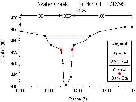
If there are multiple points with the same minimum channel elevation, the x-coordinate
(station) of the channel center is calculated by averaging x-coordinates of the points
with the minimum elevation. It should be noted that I encountered a problem in this
step due to a minor bug in the HEC-RAS (v2.1) programming. I discovered that the
cross-section coordinates in the output text file are not always space delimited.
When this occurs, a single location with the coordinates 1144.5797, 650.84 might
appear as 1144.5797650.84. When presented with a value such as this, the "RAS-Read.ave"
script will not work. To remedy this, I had to manually edit the output text file
wherever this occurs. I've brought this to the attention of Vernon Bonner who manages
the RAS programming group at HEC. Hopefully this bug will be repaired in HEC-RAS version
2.2, which is due to be released sometime in the summer of 1998. At any rate, when
all of the stream information is read from the output text file, it is subsequently
written to an ArcView virtual table. The following graphic illustrates the result.
The fields "Station No." and "Flood Elevation" are self-explanatory. The "Location"
field contains short descriptions of the cross-section location that were input in the
original geometry file for certain cross-sections. "Channel Y" shows the distance
along the stream starting at the upstream end. The remaining fields contain the left
and right widths of the floodplain and bank stations, as measured from the center of
the stream. The table is saved in database format (dbf), so it could be opened in
Excel and Access in addition to ArcView. However, all that has been done in this step
is to transform data in text file format to dbf format. Absent from this table is a
shape field; the cross-section data still must be geographically referenced.
The next step is to assign geographic coordinates to the cross-sections. This can be
accomplished by linking the RAS stream to the same stream in DLG format. For this
project, I obtained a subset of Rf3-Alpha from the
Center for Research in Water Resources (CRWR) at U.T.'s J.J. Pickle Research Campus.
Rf3-Alpha may still have some bugs and hence, it's not yet widely available. The river
reach files can be quite large. For example, Rf3-Alpha for the Hydrologic Unit Code
(HUC) representing part of Austin consists of 2.7 megabytes. As such, it would be
advantageous to work only with the stream information relating to the RAS modeled stream.
To this end, I've written a second script, "RASriver.ave", that creates a new shapefile
from selected polyline(s) within a larger coverage. A polyline is an ArcView term which
refers to a single continuous line composed of numerous individual line segments joined
at vertices. The first and last vertices are referred to as the "from" and "to" nodes,
respectively, giving a property of direction to the stream representation. Once the stream
coverage has been added to the view window, the stream (polyline) of interest is chosen
with the mouse by first clicking on the select tool  and then on
the stream. The result should look something like this (the selected stream is highlighted
in yellow):
and then on
the stream. The result should look something like this (the selected stream is highlighted
in yellow):
Next, invoke the "RASriver.ave" script by clicking the  tool in
the view window and a new, and considerably smaller shapefile is created. The original
Rf3-Alpha shapefile can now be deleted from the view. Currently, the "RASriver.ave"
script performs a similar function as the Theme/Convert to Shapefile menu option
in the view window, but I plan to modify it in the future to allow the selection more
than one stream segment, as long as a continuous line results when the segments are
put together (i.e., no branches).
tool in
the view window and a new, and considerably smaller shapefile is created. The original
Rf3-Alpha shapefile can now be deleted from the view. Currently, the "RASriver.ave"
script performs a similar function as the Theme/Convert to Shapefile menu option
in the view window, but I plan to modify it in the future to allow the selection more
than one stream segment, as long as a continuous line results when the segments are
put together (i.e., no branches).
Before adding the cross-sections to the view, the length of the RAS modeled stream
versus that of the Rf3 stream must be evaluated. It is entirely possible for example,
that the Rf3 stream is defined to a point farther upstream than the RAS stream, or
vice versa. Hence, it is necessary to define the upstream and downstream boundaries
of the RAS stream in the view window. To this end, I've written a third script for
this project named "addpnt.ave", with which the upstream and downstream boundaries
can be established with a click of the mouse. To invoke the script from the view
window, click the  tool prior to defining the upstream boundary
and the
tool prior to defining the upstream boundary
and the  prior to defining the downstream boundary. When a
point is clicked, the script determines the nearest point along the stream polyline
and snaps the point to the stream. In this way, it is guaranteed that the boundary
points fall exactly on the stream polyline. A new polyline can now be established,
with the upstream and downstream boundary points defining the "from" and "to" nodes,
respectively. Often, the boundary points are more easily pinpointed by comparison
to the location of an existing structure (e.g., road, bridge, etc). The GIS format
allows a coverage of such a structure to be easily overlaid to assist in the boundary
points selection process. Following definition of the stream boundaries, the view
might look like this (the boundary points are depicted in green):
prior to defining the downstream boundary. When a
point is clicked, the script determines the nearest point along the stream polyline
and snaps the point to the stream. In this way, it is guaranteed that the boundary
points fall exactly on the stream polyline. A new polyline can now be established,
with the upstream and downstream boundary points defining the "from" and "to" nodes,
respectively. Often, the boundary points are more easily pinpointed by comparison
to the location of an existing structure (e.g., road, bridge, etc). The GIS format
allows a coverage of such a structure to be easily overlaid to assist in the boundary
points selection process. Following definition of the stream boundaries, the view
might look like this (the boundary points are depicted in green):
Now that the stream boundaries have been established, the cross sections can be
added between them. In this step, the length of the RAS modeled stream versus that
of the Rf3 stream between the boundary points is important. I've termed this the
"lengths ratio." By establishing the boundary points in the first place, the lengths
ratio should be nearly 1, but likely not exactly 1. If the RAS stream length exceeds
the Rf3 stream length, the reach lengths between cross-sections will need to be
compressed by the lengths ratio. In contrast, if the RAS stream length is less than
the Rf3 stream length, the reach lengths between cross-sections should be expanded.
In this manner, the proportionality of RAS reach lengths is preserved. Once this re-
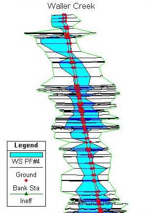
sizing is complete, the cross-sections can be laid out along the stream:
The cross-sections have been added through the use of a fourth script I've written
called "convert.ave." The script has been attached to the  tool in the view window. The width of the left and right floodplain at each cross-
section comes from the ArcView table containing the stream geometry data previously
extracted from RAS. The location of any given cross-section along the stream is
determined by multiplying the river station by the lengths ratio prior to normalizing
by dividing by the length of the Rf3 stream (as defined by the boundary points). The
result is the location of the cross-section that is expressed as a percentage of the
Rf3 stream length. At this point, the location of the cross-sections are known, but
not the orientation. To determine this, it is assumed that the cross-sections occur
in straight lines, perpendicular to the stream. The slope of the stream was determined
using points immediately upstream and downstream of the cross-section. The slope of
the perpendicular line was subsequently calculated by taking the negative inverse of
the stream slope. With the cross-section locations and orientations now known, a
line representing the floodplain at each cross-section could be added. A closer look
of the cross-sections looks like this:
tool in the view window. The width of the left and right floodplain at each cross-
section comes from the ArcView table containing the stream geometry data previously
extracted from RAS. The location of any given cross-section along the stream is
determined by multiplying the river station by the lengths ratio prior to normalizing
by dividing by the length of the Rf3 stream (as defined by the boundary points). The
result is the location of the cross-section that is expressed as a percentage of the
Rf3 stream length. At this point, the location of the cross-sections are known, but
not the orientation. To determine this, it is assumed that the cross-sections occur
in straight lines, perpendicular to the stream. The slope of the stream was determined
using points immediately upstream and downstream of the cross-section. The slope of
the perpendicular line was subsequently calculated by taking the negative inverse of
the stream slope. With the cross-section locations and orientations now known, a
line representing the floodplain at each cross-section could be added. A closer look
of the cross-sections looks like this:
The magnified view gives a better picture of the orientation of the floodplain at each
cross-section. However, it also indicates that some of the cross-sections intersect,
an occurrence that likely does not accurately represent reality. This is infidelity is
likely due to the method for determing the slope of the stream channel. A better approach
might be to calculate the slope using a greater portion of the stream, rather than
strictly the points immediately upstream and downstream of the cross-section of interest.
This would involve using a curve fitting algorithm, but it would generate a slope that
was more representative of the general shape of the stream (the effects of sharp bends
would be removed).
To complete the goal of displaying the floodplain in a GIS, much work remains to be
completed. These tasks will likely involve the following:
- Script Refinements. Throughout this report, I've indicated some
ideas for script refinements. These include editing "RASriver.ave" to accept more
than one stream segment and editing "convert.ave" to include a better method for
determining cross-section orientation.
- Floodplain Evaluation. The eventual goal of the project is to
produce a representation of the floodplain for a given flood event. This will involve
summing the individual floodplain lines to produce a single floodplain polygon. Then
the floodplain coverage could be laid over a coverage of structures of interest (e.g.,
homes, business, roads) so that flooding impact could be evaluated.
- Digital Orthophotographs. Digital orthophotos are aerial photographs
in which distortions caused by camera tilt and relief have been removed. The resulting
image is a true scale photographic map. For this project, orthophotos of the stream
vicinity could be used as a base map upon which the floodplain coverage could be overlain
and compared. In this manner, areas inundated by flood waters could be visualized.
| Data | Feature | Class |
Units | Description |
|---|
| waller.g05 | Waller Creek geometry | Text file |
Distance measured in feet | Existing channel geometry compiled from survey
information |
| waller.f10 | Waller Creek existing flows | Text file |
Flow rates measured in cubic feet per second | Flow profiles based on current
land use |
| 205_st | EPA River Reach File 3 (Alpha) | Polyline |
Distance measured in feet | Vector stream coverage for Austin (HUC 12100205) |
| Roads | Road coverage | Line |
Distance measured in feet | Vector road coverage of Austin |
 Return to Eric Tate's home page