SWAT in EPA's BASINS 3.0
and the Austin-Travis
Lakes Cataloging Unit
CE394K.2 Surface Water Hydrology
Final Report
Kristina Schneider
CE 394K.2
![]()
References
![]()
Introduction
EPA's BASINS 3.0 program is currently available in Beta release to the public. This project uses the Beta release available to the public and a follow-up Beta version made available to CRWR from the EPA. The complete release was to be available this spring but due to errors found in a final round of testing the full release of BASINS 3.0 will not be available before the deadline of this project. However, it is planned when the final release of the program is available to the public, a complete study of this area will be made.
The intent of the project was to investigate BASINS 3.0's ability to model the hydraulic and water quality conditions of Lake Austin. Lake Austin is located below Tom Miller Dam and is part of the Lower Colorado River Basin (See the map below). It is a vital part of the City of Austin and has great recreational uses. In addition, it is the water body directly upstream from the intake of the Davis Water Treatment Plant that provides part of the City of Austin's drinking water. This water is designated for the calculation of a TMDL for organic enrichment and low dissolved oxygen.

Source: LCRA website
After further investigation of the capabilities of BASINS, it was determined that a study of the entire Cataloging Unit (CU), in which Lake Austin is located, would be more appropriate. A cataloging unit is a geographic area representing all of a surface drainage basin, a combination of drainage basins, or a distinct hydrologic feature. It is the currently smallest hydrologic unit defined by the USGS's hydrologic classification system. The CU studied is 12090205, Austin - Travis Lakes. The specified goals for this project are to understand the application of SWAT in BASINS 3.0 for water quality model and to apply the model to the Austin - Travis Lakes CU.
![]()
First, the question to be asked is what is a TMDL. TMDL stands for Total Maximum Daily Load. It is both a calculation of the maximum amount of a pollutant that a water body may receive, as prescribed by a water quality standard, and an allocation of this load between the users of the water body. The load allocation takes into account the pollutant amount contributed by point and non-point sources as well as considering a margin of safety. Seasonal variation in the pollutant is also accounted for in the TMDL. The following equation presents a mathematical representation of the TMDL.
WLA = Load Point Sources + Load Non-point Sources + Margin of Safety
The standards are set by the states and it is also the states that determine which waters are impaired enough to justify an TMDL. The waterbodies designated for a TMDL are named on the 303 (d) listing as prescribed by the Clean Water Act.
The Austin-Travis Lakes Cataloging Unit is located in central Texas and extends from Burnet in the northwest corner to Austin in the southeast and covers 1251.06 sq mi. The northwest corner of the watershed is rural, while the southeast portion contains the urban area of Austin. A map provided by the EPA on the Surf Watershed website is located below.

Several waters in the CU have been listed by the TNRCC (Texas Natural Resource Conservation Commission) on the 303 (d) list. There are five of these waterbodies in the Austin-Travis Lakes Cataloging Unit. The following map and table present the waters selected and for which contaminants a TMDL will be created.

| Listing state | ID | Waterbody | Parameter of Concern | Priority for TMDL development | Is the Waterbody Targeted for TMDL development before the year April, 2000? | Potential sources of Impairment |
|---|---|---|---|---|---|---|
| TX | TX-1403-1998 | LAKE AUSTIN | ORGANIC ENRICHMENT/LOW DISSOLVED OXYGEN |
LOW | No | POINT SOURCE, |
| TX | TX-1427-1998 | ONION CREEK | TOTAL DISSOLVED SOLIDS |
LOW | No | NONPOINT SOURCE, POINT SOURCE, |
| TX | TX-1428-1998 | COLORADO RIVER BELOW TOWN LAKE | PATHOGENS |
MEDIUM | No | NONPOINT SOURCE, POINT SOURCE, |
| TX | TX-1429-1998 | TOWN LAKE | CHLORDANE PATHOGENS |
MEDIUM | No | NONPOINT SOURCE, |
| TX | TX-1430-1998 | BARTON CREEK | PATHOGENS |
MEDIUM | No | NONPOINT SOURCE, |
Source: http://www.epa.gov/iwi/303d/12090205_303d.html
BASINS stands for Better Assessment Science Integrating Point and Non-point Sources and was developed to aid in the determination of TMDLs. The BASINS programs are designed to investigate water quality conditions in water bodies and in themselves are not models. BASINS provides an interface that allows the user to interact with point and non-point source pollution models in GIS based environment. The program Arc View is utilized to upload GIS data from the BASINS database, which is provided by EPA’s Office of Science and Technology. The four models available with BASINS 3.0 are SWAT, QUAL2E, PLOAD, and WinHSPF. GenScn is a program provided to interpret the outputs from WinHSPF and SWAT. In addition, BASINS 3.0 contains several new functions, which include an automatic delineation tool that uses DEMs to create watershed boundaries, a NHD-import tool that downloads and formats the NHD from the web, and a watershed report function for land use, topography, and hydrologic response units.
The BASINS database provides the data input for all the models, which include base cartographic data, environmental background data, environmental monitoring data, and point sources/loading data. BASINS 3.0 also contains several new data types, one of which is 1-degree DEM grids. Currently data for only one cataloging unit, HUC-05010007, in Pennsylvania has been formatted completely for the BASINS 3.0 format. The flow chart below demonstrates clearly the components of BASINS 3.0.
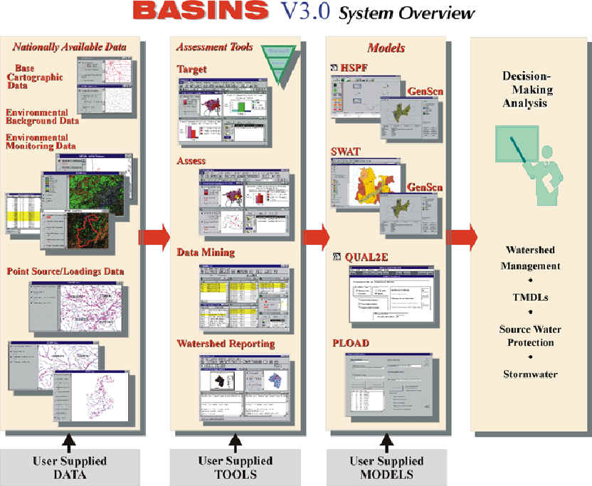
Source: BASINS 3.0 User Manual
Another interesting feature of BASINS 3.0 is that it is packaged in a different format from previous versions. The program is distributed as a core system and several ArcView extensions. All BASINS components, such as the assessment tools and models, are presented as extensions. This allows users to only add the extensions that are needed. Also, from a maintenance standpoint this structure is advantageous since individual extensions are easier to maintain and update because patches do not need to be provided for the entire program. The new BASINS 3.0 provides a streamlined program structure as well as better data sources and models in comparison to older versions.
![]()
SWAT stands for Soil and Water Assessment Tool and is a public domain model supported by the USDA Agricultural Research Service at the Grassland Soil and Water Research Laboratory. It is a watershed scale model intended to model the effects of land management practices on large complex watersheds. In addition, the effects of varying soil types and land uses on the watershed can be interpreted. SWAT is a long term yield model that is not designed to model single event flood routing. As a long term yield model, it allows for the study of long-term impacts of pollutant loading, such as the gradual buildup of pollutants.
The model is physically based, meaning the effects of changes in management practices, climate, and vegetation as well as watersheds without stream gage data can be modeled. Another benefit of using SWAT in BASINS 3.0 is SWAT allows the user to model decades of natural processes for which, the model requires a large amount of input data. The input data is largely already in the BASINS databases and it must only be formatted correctly, which BASINS does.
SWAT models the hydrology of the watershed with the following components:
Evapotranspiration: The evaporation from soils and plants are modeled differently. Potential evapotranspiration can be estimated with three methods: Hargreaves, Priestley-Taylor, and Penman-Montheith. Actual soil water evaporation is calculated using exponential functions of soil depth and water content. Potential evapotranspiration and a leaf area index is used to estimate the potential soil water evaporation and the plant water evaporation.
Percolation: A storage routing technique combined with a crack-flow model is used to predict the flow through each soil layer. The cracked flow model allows for the percolation of infiltrated rainfall, though the soil water content is less than field capacity. The portion of the rainfall that becomes part of the stored water cannot percolate until storage exceeds field capacity.
Lateral Flow: Lateral flow is defined as the stream flow contribution below the surface but above the saturated zone. It calculated simultaneously with percolation using a kinematic storage model that allows for flow upward. The model accounts for variation in conductivity, slope and soil water content.
Groundwater Flow: The portion of the groundwater that contributes to the stream flow is called return flow. It is simulated by a shallow unconfined aquifer that is replenished by the moisture in the soil profile. The flow from the aquifer to the stream is delayed using a recession constant, calculated from the daily stream flow records. In addition to the shallow aquifer, a deep confined aquifer is simulated to allow for percolation from the upper aquifer. Pumping may also be used to remove water from the shallow aquifer.
Surface Runoff: The model calculates both runoff volumes and runoff rates. The runoff volume is found using a modification of the SCS curve number method. The SCS method was chosen since it is reliable and has been in use for many years in the US. In addition, it is computationally efficient and requires readily available inputs. Finally, it relates runoff to soil type, land use, and management practices. The modification deals with CN value, which varies non-linearly. The peak runoff rate is calculated with a modified Rational Formula. A stochastic technique is used to calculate the rainfall intensity, and the runoff coefficient is determined by dividing the runoff volume by the rainfall. Finally, overland and channel flow are used to find the time of concentration.
Ponds/Reservoirs: The storage in these waterbodies is estimated using the capacity, inflows, outflows, seepage and evaporation. It is assumed only emergency spillways exist.
Transmission Losses: Semiarid watersheds often have alluvial channels that remove large volumes of runoff. The Lane method from the SCS Hydrology Handbook is used to calculated these losses.
It is interesting to note that SWAT separates soil profiles into 10 layers to model the inter- and intra-movements between the layers. The model is applied to each soil layer independently starting at the upper layer.
To model a watershed in question, the watershed is broken into subbasins. This allows for the consideration of variations in land use and soil type and how they effect the hydrology of the system. In addition, the subbasins allow different areas of the watershed to be related spatially. The following categories are used to organize the input information for the subbasins: ponds/reservoirs; groundwater; weather and climate; HRUs; and the main channel draining to the next subbasin. An HRU is a hydrologic response unit that is a unique combination of soil, land use, and management practices.
With an understanding of both the components of the SWAT model and the area of study, the next step is to apply the model. The first thing that is needed is the input data for the model. Since BASINS data for only one CU in Pennsylvania has been reformatted for BASINS 3.0, the data from BASINS 2.0 was used. It is possible this may cause some problems since the formats for some files are different but hopefully problems will be minimal. This data was downloaded from the EPA BASINS website. Next to apply the model, multiple steps are involved. The process of using SWAT in BASINS 3.0 is listed below:
Activate SWAT, the Automatic Watershed Delineator, and Land Use, Soil Classification, and Overlay Extensions.
Delineate the watersheds
Define the Land Use and Soils
Define the HRUs (Hydrologic Response Units)
Define the weather data
Apply the default input files writer
Set-up (requires specification of simulation period, PET calculation method, etc.) and run SWAT.
Interpret the output data using GenScn.
To activate SWAT and it's needed extensions, you simply go to the BASINS extensions area in ArcView and select the needed extensions. The following graphic shows the model extension category. Extension categories exist for watershed delineation tools, reports, and assessment tools to name a few.

To delineate the watersheds, the subbasins as explained above, two options are available. One is a manual watershed delineation tool and the other an automatic version. The automatic version was utilized in this project. This step is a very important step that determines the success of future phases of the model application. The screen shot below shows the interface for the automatic watershed delineation tool.

The first step is to select a DEM grid. The DEM provided with the BASINS 2.0 is a polygon, therefore Spatial Analysis was used to convert the polygon to a grid. The value used for the grid was the elevation in meters. The focusing watershed area creates a buffer, designating the area of the DEM that should be used to delineate the subbasins. The outline of the CU was used as the focusing area. The burn-in option allows user to specify a shapefile that will direct the flow from the DEM to the correct location. The reach file of the NHD was converted into a shape file and then was selected as the stream that would be burned in to the DEM. However, some errors were encountered in the delineation of the watersheds with this DEM. The program has a step in the delineation process that creates the streams that will be used in later parts of the delineation. The DEM available was not exact enough to allow for the creation of the streams that followed the NHD. The following image is an example of the problem. The bright blue lines are lines created by the delineation 78749tool and the light green lines are the NHD shapefile.

To deal with this problem it was decided to use the NED 1 degree DEM, which has cell sizes of 30 m by 30 m. However, the NED DEMs are not in the same coordinate system as the BASINS data and more problems arose from attempts to project the data.
A solution was found that allowed for the delineation of the watersheds. In the previous conversion of the BASINS 2.0 DEM polygon to a grid the analysis extent had not been detailed. The analysis extent specifies the window that will be used for calculations with Spatial Analyst. The image below shows the Analysis Properties interface that allows for the definition of the analysis extent.

In addition to specifying the extent of the analysis, the analysis cell size was set the same as the NED DEM. This created more cells in the new grid created from the BASINS 2.0 polygon, which created a more detailed DEM. This DEM was specific enough to allow for the delineation of the subbasins. Just one other file had to be modified to allow for the delineation of the watersheds. At the outlet of the cataloging unit the NHD shapefile did not flow out of the CU but formed a v shaped loop that did not allow for flow out of the cataloging unit. The shapefile was edited to split the line and direct the lines outside the CU. The figure below shows that the shapefile and the changes made to allow for watershed delineation.

With these changes made, the entire watershed delineation proceeded without problems. The resulting watersheds are shown below.

•
One interesting thing to note in this figure is that only two of the subbasins are labeled, 1 and 0. In addition, the attributes of the subbasins are all given values of zero except for subbasin 1 as can be seen below.

This is a bit strange but this fact was overlooked to continue the investigation of SWAT's capabilities in BASINS 3.0.
With the watersheds delineated it is now possible to format the land use and soil inputs for the model. The Land Use and Soil Definition Utility as well as HRU distribution tool are now available for use.

As described in the model overview the land use and soil distribution is an important factor in the application of SWAT. The Land Use and Soils Classification and Overlay tool is helpful in loading the land use and soil data, which is then placed in the current projection. The data can be in either a grid or a shapefile. For the delineated watershed the land use soil combinations and distributions are determined. Once this is complete the HRUs can be calculated. The image below shows the interface with an explanation of the fields and actual data input. Also, the Land Use and Soil grids created are shown below.


The next step is to compute the Hydrologic Response Unit distribution. The HRU distribution utility allows the user to specify the criteria for determining the HRU division throughout the subbasin. The interface for this step is located below. Each subbasin can have one or more HRUs. Either the dominant land use and soil in the subbasin can be used or HRUs can be defined based on the percent land use over the subbasin and the soil class percent over the land use area.


The preliminary work is done and SWAT is available!

Once in the SWAT View, the weather data can be stipulated and the input writer can be utilized to build the watershed input values. The weather data generation allows the user to input their own data or simulation data. Weather data from a US database contains default data from nearby weather stations.

Creating the watershed input values is the first step in running SWAT. The program allows the user to write all files or to individually write the files. The status of the input files is tracked with Current Status of Input Data message box, when a file is complete a check box is placed next to the file.


This is the point in the procedure when the strange delineation of the watersheds came into play. The soil input file could not be created because data was missing for multiple soil types. The data exists in the soil tables used to create the Land Use and Soil overlay but not in the report created by the Land Use and Soil distribution, which is used to generate the .sol file. The report is shown below and it can be seen that only nil values exist for subbasin 0, while subbasin 1 is correctly calculated.

The reason for this miscalculation most likely stems from the imperfect delineation of the subbasins. The area of the subbasins are used to determine the percent of the area that the land use and soil types cover. Since, the calculated area for subbasin 0 is zero then of course the percent of area with a certain land use will be zero. The soil input will logically not accept a value of zero for the area a soil type covers, an error occurs and the input files cannot be correctly written. This was the final step of the process that was attempted.
![]()
One of the goals of this project was to model the hydrologic and water quality conditions in the Austin-Travis Lakes CU with SWAT in BASINS 3.0. This goal was not achieved but it was not the top priority of the project. The main goal was to become familiar with the steps and processes associated with the modeling of the Cataloging Unit with SWAT. This goal was achieved and much was learned about the nature of the input data that is necessary for a correct run of the program. It is vital the delineation of the watersheds be correct because future calculations are based on the delineation. In addition, the data used to delineate the watersheds must be precise enough to create the subbasins.
One important detail that must be taken into consideration when analyzing the results of this project is that the model used was a beta version. Once the completely tested version is available it is highly possible that the issues encountered will be nonexistent. Also, the data used for this study was formatted for BASINS 2.0. It is highly possible that the delineation error occurred because the DEM had to be converted from a polygon or certain unspecified files are missing from the BASINS 2.0 data format. When both the final version of BASINS 3.0 and the correctly formatted data is available the application of the model will run much smoother. It is planned to use the final version when it becomes available to model nutrient loading in the Austin-Travis Lakes CU.
This project has shown the possibilities that SWAT provides for the calculation of nutrient transport and pesticide transport are rather remarkable. The model is physically based allowing for a greater understanding of what is occurring hydrologically in watershed. Also, the ability to model long time periods provides for simulations that can be used for long range planning. For the creation of TMDLs, the ability to plan far into the future is a needed benefit. Great possibilities exist for the use of SWAT and BASINS 3.0.
![]()
References
BASINS 3.0 Web page: http://www.epa.gov/ost/ftp/basins/system/BASINS3/areadb3.htm
SWAT User Manual: Model Components http://www.brc.tamus.edu/swat/usermanual/modelcomponents.html
SWAT User Manual Theortical Documentation: http://www.brc.tamus.edu/swat/swattheo.html
![]()
Interesting Related Sites
SWAT Home Page: http://www.brc.tamus.edu/swat/index.html
Surf Your Watershed, Austin-Travis CU: http://www.epa.gov/surf3/hucs/12090205/
EPA TMDL Home Page: http://www.epa.gov/OWOW/tmdl/index.html
Enviromapper for Watersheds: http://map2.epa.gov/enviromapper/
![]()
Special Thanks
Dr. Mauro DiLuzio, Blacklands Research Center
Dr. Raghavan Srinivasan, Blacklands Research Center
Paul Cocca, BASINS Team US EPA Office of Water
Dr. Francisco Olivera, Center for Research in Water Resources
Vicki Samuels, Center for Research in Water Resources
My Editor