presented by: Victoria Samuels, vsamuels@mail.utexas.edu
presented for: CE 394K.2 Surface Water Hydrology, Spring 2001

One of the main objectives of the Texas Water Development Board (TWDB) is to study and determine how much water will be needed to maintain Texas's streams, rivers, bays and estuaries. This program is being investigated concurrently by the TWDB, the Texas Parks and Wildlife Department and the Texas Natural Resource Conservation Commission (TNRCC). In this study, monitoring data and studies will be compiled to evaluate the needs for instream flows and freshwater inflows to estuarine systems in Texas. Unfortunately, many of the coastal watersheds are ungaged and difficult to model and simulate with traditional rainfall/runoff models.
|
|
|
In order to study the flows from the ungaged watersheds, TWDB developed a program known as TxRR, the Texas Rainfall-Runoff Model. The model determines calibration factors for a particular TWDB gage watershed based on a genetic algorithm optimization technique. The calibration factors match the modeled runoff from the given precipitation file to the observed runoff from the input runoff file, on a daily basis. The procedure analyzes the soil moisture of the area continuously and direct runoff on an event by event basis.
Once the calibration factors are determined, they are related to an ungaged watershed with the relationship:
SMMAXU = (CNG/CNU) * SMMAXG
where the U represents the ungaged watershed parameters and G represents the gaged watershed parameters. CN is the curve number of the specific watershed. SMMAX is the maximum soil moisture of the watershed, which will be explained further in the Water Balance discussion. This relationship makes sense because the curve number acts as an indicator of soil retention and the ratio of CNs is inversely proportional to the soil retentions.
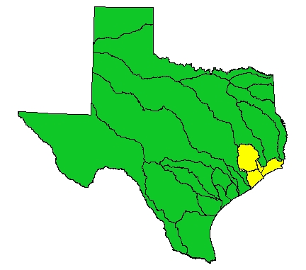
The study area used for this work derives from my research efforts for the TNRCC, evaluating water quality management segment watersheds in Basin Group C in Texas. Basin Group C is located on the Eastern coast of Texas, surrounding the Houston area.
|
The State of Texas, with Basin Group C highlighted |
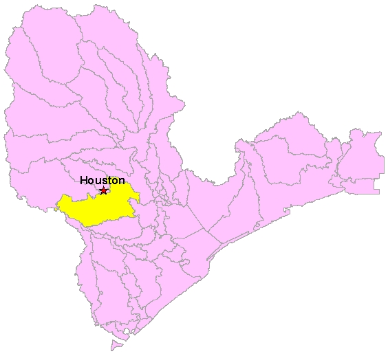
Basin Group C, with watershed #1007 highlighted |
My research task was to partition the landscape of Basin Group C into watersheds for each of the designated segments. Because Basin Group C is comprised of 3 coastal basins and a river basin, the region is very flat and presented a challenge for watershed delineation. However, these issues make it a prime candidate for use in the TxRR model, which is designed for use in coastal areas with ungaged watersheds.
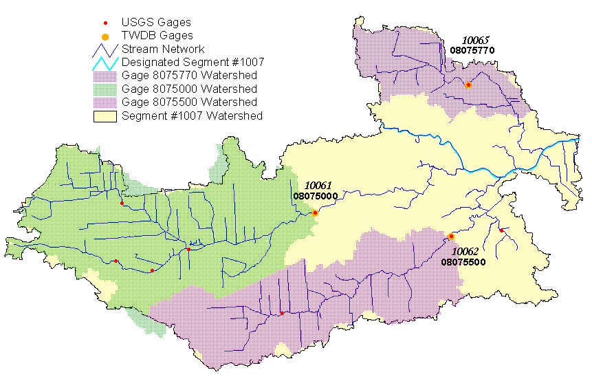
The main factor dictating the study area choice is the availability of precipitation and runoff data in the TxRR format. Currently, only TWDB gages have data in the TxRR format. Therefore, it was necessary to chose a watersheds for TWDB gages. Many TWDB gages are coincident with USGS gages, that already have drainage areas delineated. In comparing the USGS gages and the TWDB gages, three gages are represented by both agencies in the Buffalo Bayou Tidal (Segment #1007) watershed near Houston. The Water Availability Modeling (WAM) project, organized by TNRCC and performed by CRWR, has determined watersheds for these gages and other control points in the area. These WAM drainage areas can be merged to determine the watershed for the gage. These watersheds all fall within the watershed for segment #1007. These three watersheds became the initial study area for this model calibration effort.
|
Segment #1007 Watershed, with the three selected gages for study highlighted. The top script number is the TWDB gage identifier and the bottom print number is the USGS gage identifier. The individual gage watersheds were obtained from WAM and do not directly correspond to the gages obtained now. |
The drainage areas of the gages was found at the USGS website, http://water.usgs.gov/tx/nwis/sw and confirmed by the WAM results. They are as follows:
| TWDB Gage No. | USGS Gage No. | USGS Gage Name | Drainage Area (sq mi) |
| 10061 | 8075000 | Brays Bayou at Houston | 94.9 |
| 10062 | 8075500 | Sims Bayou at Houston | 63.0 |
| 10065 | 8075770 | Hunting Bayou at IH 610 | 16.1 |
My objectives for this project changed throughout the course of the work. First, my goal was to "play around with the model". Because there has been no significant attempt to calibrate the model at CRWR, I planned to determine the effects of altering various input parameters in the model. After determining the effects of the parameters, I planned to find the best fit match possible between the modeled and actual runoff hydrograph for the three gaged watersheds. Because these gaged watersheds are all within the same TNRCC Water Quality Management watershed, I assumed that their characteristics are similar. To test this assumption, I planned to use the calibrated parameters from the other two watersheds and evaluate the modeled runoff hydrographs, possibly using statistical analysis.
However, during the calibration effort, numerous results were not as I expected, and led me to abandon my original objectives of comparing the calibrated parameters for the three watersheds. Rather, I chose to study only two of the watersheds, for gages 10061 and 10062, and employ the gaged/ungaged watershed relationships that reflects the model's purpose. These are the efforts described in this paper.
The TxRR model was developed as a compilation of hydrological models and methods. These include the Agricultural Research Service (ARS), the Soil Conservation Service (SCS) Curve Number method, parameter optimization using Newton's Method and the SCS Unit Hydrograph. However, the model has evolved from these systems through various changes. The ARS model uses only one annual soil moisture depletion factor, while TxRR employs 12 monthly depletion factors. The parameter optimization now utilizes Genetic Algorithms rather than Newton's Method. The output hydrograph also assumes the shape of a Gamma function, rather than the SCS Unit Hydrograph.
As in all hydrologic models, the core of the model is the approach to the water balance. A brief discussion is given here, and the equations and processes can be seen in more detail in the following presentations:
The water balance for TxRR is as follows:
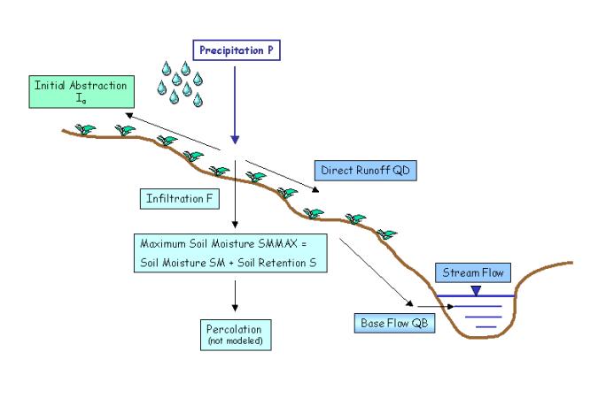
TxRR Water Balance
The time frame for TxRR is also unique in that it considers precipitation events as in "i" space, while it considers each parameter at the time before and after each individual precipitation event as one time increment and the time between precipitation events as a separate time interval. The following figure attempts to clarify the time variables within the TxRR water balance equations, described below.
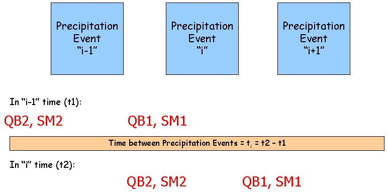
TxRR Time Variables
The sequence of the model is as follows:
Before precipitation event ''i", the soil moisture SM depletes from the end of event "i-1" to the beginning of event "i" using the equation: SM2i = SM1i-1 exp (-amti) in which am is the monthly depletion factor for month m. The baseflow QB also receeds from the end of event "i-1" to the beginning of event "i" based on the equation QB2 = QB1 * Kt2-t1
After the soil moisture depletes, the new soil retention Si is calculated as Si = SMMAX - SM2i in which SMMAX is the maximum soil moisture, optimized by the model
It Rains! Pi (precipitation) at time ti
The direct runoff QD is calculated with the following equations: QDi = Pei2/(Pei + Si) in which Pei is the effective precipitation determined from the equation Pei = Pi - Iai, in which Iai is the initial abstraction, found from the equation Iai = abst1 * Si, where abst1 is the initial abstraction coefficient (usually 0.2)
The new soil moisture is computed by SM1i = SM2i + Fi in which Fi is the infiltration found from the equation Fi = Pi - Iai - QDi
The new baseflow from the precipitation event is calculated based on one of two equations: QBnew = wB * Pi * (SM2i/SMMAX) or QBnew = wB * Fi * (SM2i/SMMAX) in which wB is the baseflow coefficient or weighting factor.
The final baseflow after precipitation event "i" is calculated as QB1i = QB2i + QBnew
Several terms and definitions should be explained:
|
Soil retention is the dry space in the soil column, essentially the room available for additional moisture or an abstraction. |
|
|
Baseflow is the part of the streamflow that flows out long after a precipitation event. It can be either groundwater runoff, subsurface runoff, or a combination of the two. |
|
|
The equations to determine the new baseflow are using the assumption that the baseflow increment is proportional to either the amount of precipitation or infiltration. It is also related to soil moisture because the baseflow is larger when the soil moisture is larger. |
|
|
In choosing which new baseflow equation to use, the infiltration equation is considered more conceptually correct. However, as the infiltration approaches zero, this leads to the new baseflow to also be zero, even if the precipitation event yields a large amount of rain. This would occur if the initial abstraction or soil retention is large enough to hold all of the precipitation. If it is realistic that the initial abstraction or soil retention is that large, then the infiltration equation should be used. If it is not likely that the initial abstraction or soil retention can hold the entire precipitation event, then the precipitation equation should be used. |
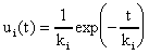
The routing mechanism used by TxRR, upon replacement of the SCS Unit Hydrograph, is a series of identical, completely mixed, linear reservoirs, represented by the gamma function. Two main variables characterize a cascade of linear reservoirs, "ki" the detention time of each reservoir, and "Ni", the number of reservoirs in the cascade.
The foundation for this approach is the linear reservoir model, in which a reservoir of detention time ki has a redistribution function ui(t):
Redistribution refers to the distribution of the output, given the input. In a series of linear reservoirs, this output is then cycled into another reservoir as the input, and the redistribution function is applied to itself. The general result of this method is the following redistribution function:
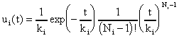
This scenario only allows for the number of reservoirs to be an integer value. However, because this is an approximation technique, Ni can be any real value. Therefore, the quantity (Ni - 1)! is replaced by the gamma function G(Ni) in the following equation:

In evaluating the appearance of the gamma function distribution, multiple values of N and k were used. The following graph displays the results:
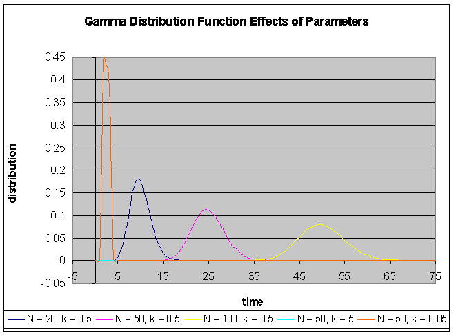
From this graph, these relationships can be determined:
|
When k is constant, as the number of reservoirs (N) increases, the peak decreases and occurs later, and the distribution spreads out farther. (see the navy, pink and yellow functions) |
|
|
When N is constant, as the detention time (k) increases, the peak decreases drastically and occurs later, and the distribution spreads out vastly. (see the orange, pink and turquoise functions) |
These relationships will be incorporated into the trial and error process of model calibration.
Genetic algorithms are considered a method of "evolutionary computing" in artificial intelligence. The development of evolutionary computing began in the 1960s by I. Rechenbert in Evolution Strategies. John Holland furthered this research and developed Genetic Algorithms (GAs), described more in his book, Adaptation in Natural and Artificial Systems.
Genetic algorithms follow the survivalistic behavior of nature. Nature develops life forms at random to survive in the environment. The weaker life forms, those which do not fit the environment well, are "killed off" while the successful life forms progress on. These successful life forms are then modified and again tested in society for their successfulness. This pattern continues until the most successful life form in the tested society is found. This process is known as natural or darwinian selection.

pictures from Introduction to Genetic Algorithms, Nick Johnson
Genetic algorithms follow the biology of living organisms in determining what contributes to the life form's success in the environment. Each living organism is made up of cells. Each cell is composed of a set of chromosomes. Each chromosome consists of genes, which are blocks of DNA, and correspond to a certain trait, like blue eyes. These traits influence how successful the life form will be.
Genetic algorithms are useful for problems that are very difficult to find a solution, but easy to check solutions for their suitability to solve the problem. These problems are termed NP-complete, where NP stands for nondeterministic polynomial. Therefore, a random sampling of solutions is provided to the genetic algorithm and the most suitable solution is chosen.
The general procedure of a genetic algorithm is as follows:
The random sampling of solutions, represented by chromosomes, are compiled as a population. Each member of the population is tested for its fitness, and the weaker members are discarded, by natural selection.
Two "parent" chromosomes are then selected from the remaining population and reproduction occurs through two processes. Crossover or recombination mixes the genes from the parents to form new chromosomes, children. The new children may then undergo mutation, in which the genes are slightly changed. Because the children are genetically similar to the parents, there is inheritance of traits.
The new children are placed in the population and the fitness of each member of the population is again assessed. The fitness is defined as a measure of the success of the organism in its life.
The process repeats back to step 1 until a criteria of fitness is met by a solution.
Because the new children are derived from the best previous parents, there is a trend toward more fit children, or solutions. However, in the case that the best solution may be lost during reproduction with another parent, or solution, a principle known as elitism is employed in which one best solution parent is carried over unchanged to the new population to be tested again.
Understanding these principles, these concepts also be considering when calibrating the model.
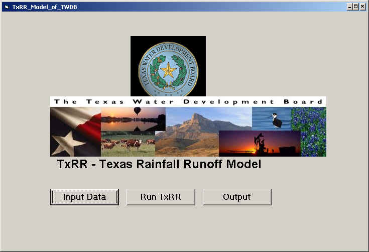
TxRR consists of three main modules: the Windows-based input screen, the DOS-based Fortran code and the Windows-based output screen. Previously, using the model would require constant shifting back and forth manually between the Windows and DOS environment; however, Venkatesh Merwade developed an interface which calls the Fortran code from Windows and eliminates this hassle.
TxRR is contained in two folders which must be installed on the C:/ drive of the computer. The first folder "TxRR" contains the Fortran code and programs to run the model. The second folder "Genalg" contains the genetic algorithm improvements to the model and houses the input data and the output file.
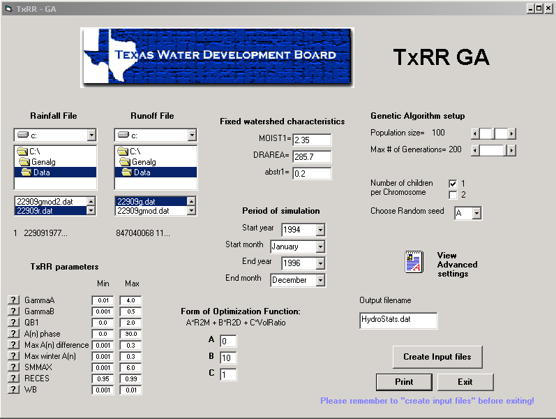
The input screen to TxRR appears daunting, with many windows which require information. However, the screen can be dissected to be much less confusing.
First, the Rainfall and Runoff Files are considered. These input files are the crucial ingredient in using the TxRR model. The rainfall and runoff files must be ".dat" files and in a format specific to how TxRR reads the data. Currently, only the TWDB has files in this format. While a program is being created to convert USGS data into this format, it is not currently available. Therefore, only gages and their watersheds from the TWDB can be evaluated with TxRR. Once the TWDB gage for study is identified, the two files must be placed in the Genalg/Data folder. Typically, the rainfall file has the suffix "r" or "pcp" and the runoff file has the suffix "g" or "gd". The two files corresponding to the user's choice of gage are then selected. For this study, the three gages of consideration and their files are: 10061_pcp.dat, 10061gd, 10062_pcp.dat, 10062gd.dat, 10065_pcp.dat, 10065gd.dat.
The next area of input data is the Fixed watershed characteristics. These characteristics deal with the gage watershed of interest. MOIST1, I assume, refers to the initial soil moisture condition. It can be used to calibrate the model, and does not appear to be scientifically derived. DRAREA is the catchment area in square miles, which was obtained from the USGS website mentioned above. The last parameter in this section is abstr1, which is the initial abstractions value. Typically this value is taken to be 0.2.
The input area Period of simulation defines what time frame will be studied. The gage data must have data for the time period selected or the model will not run. Unfortunately, when this happens, no message appears stating that this is the problem, so it is important to know if data is present for the time period.
The Genetic Algorithm setup section contains the random variables used in the genetic algorithm optimization procedure described above. It is recommended that these parameters are left as the given values initially, and can be altered for calibration purposes.
A long list of TxRR parameters appears on the input screen. However, these parameters have default ranges that are recommended for use. Therefore, these standard ranges are retained and the variables do not need to be estimated. They should be altered if the optimal solution converges on a maximum or minimum range value to ensure that the solution is not being limited by default ranges. The parameters refer to:
|
GammaA - the number of reservoirs to be used in the gamma function distribution (N) |
|
|
GammaB - the detention time to be used in the gamma function distribution (k) |
|
|
QB1 - the initial baseflow |
|
|
A(n) phase - restriction on the monthly depletion factors, which should have a sinusoidal pattern because of its seasonal nature |
|
|
Max A(n) difference - restriction on the monthly depletion factors, which should have a sinusoidal pattern because of its seasonal nature |
|
|
Max winter A(n) - restriction on the monthly depletion factors, which should have a sinusoidal pattern because of its seasonal nature |
|
|
SMMAX - maximum soil moisture |
|
|
RECES - recession constant for baseflow |
|
|
WB - baseflow coefficient |
Finally, the Form of Optimization Function refers to what sort of data is being considered. "A" corresponds to monthly data while "B" corresponds to daily data. Only one of "A" or "B" can be used. "C" relates to the volume ratio. The decision for the "best" or "optimal" solution is determined from this equation.
After filling all of the necessary input boxes, TxRR must "Create Input files" by pressing the aforementioned button. Then, exit the TxRR-GA input window. Click on the "Run TxRR" box on the main TxRR-TWDB model screen, which opens a DOS window. The code asks the user if return flow should be removed. Return flow can be used as part of the calibration techniques. If the user desires to remove return flow, the code then prompts for the universal amount to be removed from the gauged flow. If the user ignores the return flow, the code generally warns the user that over 70% of the data is zero, and this must be considered when evaluating the results.
The code then performs up to the maximum number of iterations specified in the input screen. The DOS screen should indicate the iteration number it is performing. If no DOS screen appears, then the program did not run, and the reason must be ascertained. One possible reason, as mentioned above, is that no data exists for the period of simulation selected.

Once the DOS screen has completed running iterations, click the "Output" button on the main screen. In order to view the output, navigate the menu in the lower right corner of the screen to c:\genalg\hydrostats.dat. The above hydrograph and hyetograph appear. The precipitation is shown as a hyetograph on the top of the graph, while the gauged and simulated flow are shown on the bottom of the graph. On the upper right of the screen, the parameters optimized by TxRR are listed.
Also available from output view are the Unit Hydrograph (UH) and the convergence of the genetic algorithm value (GA).
When attempting to compare results closely, the hydrographs on the output screen are not adequate to evaluate the magnitude and degree at which the gauged flow and simulated results align and contrast, as well as compare various trials. To study the results more accurately, Microsoft Excel was used by opening the Hydrostats.dat file within that interface.
CALIBRATION OF THE MODEL TO THE STUDY AREA
The initial calibration effort began as studying Gage No. 10062/8075500 (drainage area of 63.0 sq. mi.) for a three year period, January 1990 - December 1992, with no return flow removed. The results, which are optimized by design, were very different from the gauged flow. Therefore, the period of simulation was shortened, from January 1991 - June 1992, through a major storm cycle. This improved the coincidence between the modeled and gauged flow, but not by a significant enough extent. Again, the time period was decreased to the major storm sequence between December 1991-June 1992, a seven month time frame. This estimated flow had the best fit with the gauged flow but still had errors, such as overestimating a few peaks and drastically underestimating the baseflow. Therefore, the first conclusion, intuitively and though trial and error, is that a shorter period of simulation yields modeled flow that will more closely match the gauged flow. The gauged and simulated flow for December 1991-June 1992 is shown below.

After selecting a timeframe, the following parameters were analyzed for their sensitivity: return flow, Moist1, genetic algorithm information, and TxRR parameter ranges. Return flow was studied first.
Originally, the effect of removing a return flow was unknown. After several different return flow removal trials, it was determined that removing return flow decreased the gauged flow amount by the user specified return flow value, across the board. This effect was desired since the predicted baseflow was higher than the gauged baseflow and did not replicate it well. If removing return flow would decrease the gauged baseflow, this discrepancy could be reduced. Three return flow removal values were run: 50 cfs, 40 cfs, and 45 cfs. The minimum value of the gauged flow before return flow removal was 40 cfs. The three trials yielded the following results: 50 cfs had a good fit, with many peaks matching, but still overestimated at the beginning of the time period and underestimated at the end; 40 cfs had an even better fit, but still missed a few peaks by a large amount. In comparing 50 cfs with 40 cfs, 40 cfs has a better matching overall, but misses a few large peaks dramatically. However, 40 cfs has slightly less difference from the gauged flow overall. With these results, 45 cfs was removed to see if there was any intermediate effect; but, this was not noticed. Therefore, 40 cfs was removed as return flow and other calibration parameters were tried.
The next parameter modified was the initial soil moisture condition Moist1. The default value of Moist1 is 2.35. First, the Moist1 value was decreased to 1.75; however, no difference in the modeled flow was observed. Next, the Moist1 value was increased to 3.0. The effect varied across the simulation period; the peaks were raised at some times and lowered at others. Generally, the larger the peak, the greater the peak increased. This trial was a better fit to the gauged flow then the default value of 2.35 and this trend was further pursued. A Moist1 value of 4.0 was modeled. The general effect in contrast with a Moist1 value of 3.0 was a decrease in the peak values; however, in a few places, it was higher. Because the trend differed for different storm peaks, the fit of the trial was evaluated by breaking the overall simulation period into 4 periods: from December 31 - mid January, mid January - mid March, mid March - end of April, and end of April - end of June. Also, a trial with a Moist1 value of 5.0 was run. By using this focused approach to calibration, the attempt with a Moist1 value of 4.0 was chosen as the best fit.
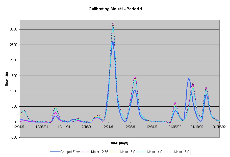 |
Moist1
of 4.0 Results:
Period 1 - same, slightly better than 3.0 Period 2 - same, good Period 3 - worse than 3.0 Period 4 - better than 3.0 |
 |
Moist1
of 5.0 Results:
Period 1 - worse than 3.0 and 4.0 Period 2 - generally the same, some peaks better, some peaks worse Period 3 - better than 4.0 Period 4 - worse than 4.0 |
Next, the genetic algorithm parameters were tested. Three parameters were considered: population size, number of children, and random seed. The population size relates to how large the initial selection of choices is, and was tested first. The default value of population size is 100, and can range from zero to 200. It was assumed that a larger population size would conceivably yield a better solution, so values greater than 100 were attempted, but no values less than 100 were tried. Again, a focused comparison was made by looking at the run results in four time periods. A population size of 200 and 150 were run, and both yielded similar, if not worse, results than a population size of 100. Additionally, the processing time increased. Therefore, the default value of 100 was retained.
The number of children was then toggled from the default 1 to 2. The results were almost identical between the two scenarios. Again, the default value of one child was used.
Lastly, the random seed was changed. It is unsure exactly what the random seed represents other than a possible starting point in the selection. Six options exist, A through F. Each of the seeds was tried and the results were evaluated. The results were looked at for each time period. Seeds B and C were not as good as Seed A. Seed D presented a better fit than Seed A and was taken as the new standard result to equal or better. Random Seeds E and F were both worse than Seed D. Therefore, Seed D was used.
These trials concluded the calibration effort for Gage 10062 for the storm season from December 1991 to June 1992. The final fit's input and output parameters are as follows:
Input
Parameters:
Output Parameters:
|
 |
Once this calibration was successful, I planned to calibrate the two other gages for the same time period. However, I quickly found out that the other two gages did not have precipitation or runoff data for the simulation period of December 1991 - June 1992. The model did not generate results because there was no data available to simulate. I then decided to use the knowledge gained for this calibration effort and quickly (a term I use loosely) calibrate the gages for the same time period. Gages 10061 and 10065 have data through December 1990. Therefore, the time period of January - May 1990 was chosen.
Again, I started with gauge 10062. I assumed that the input parameters used to calibrate 10062 for the time period 4 months later would apply to this time period with a little tweaking. However, this was found to be vastly incorrect, with the fits very misaligned. The peaks were far overestimated, ranging from an average of two times greater than the gauged value up to ten times greater than the gauged value. Therefore, several of the estimated factors were then modified in turn to see any effect on the simulated flow.
The minimum gauged flow value was found to be 35, so the first change was that the 40 cfs was not removed, considering that it would remove more than was initially there in some instances. However, this did not have any tangible effect on the flow simulation. Because the peaks were exceptionally high, the Moist1 value was decreased with the hope of decreasing the peak magnitude. Multiple scenarios were tried with Moist1 values of 2.35, 1.5, and 0.5, all using Random Seed D and no return flow removed. The following figure shows the effects of the changes in the simulated flow.
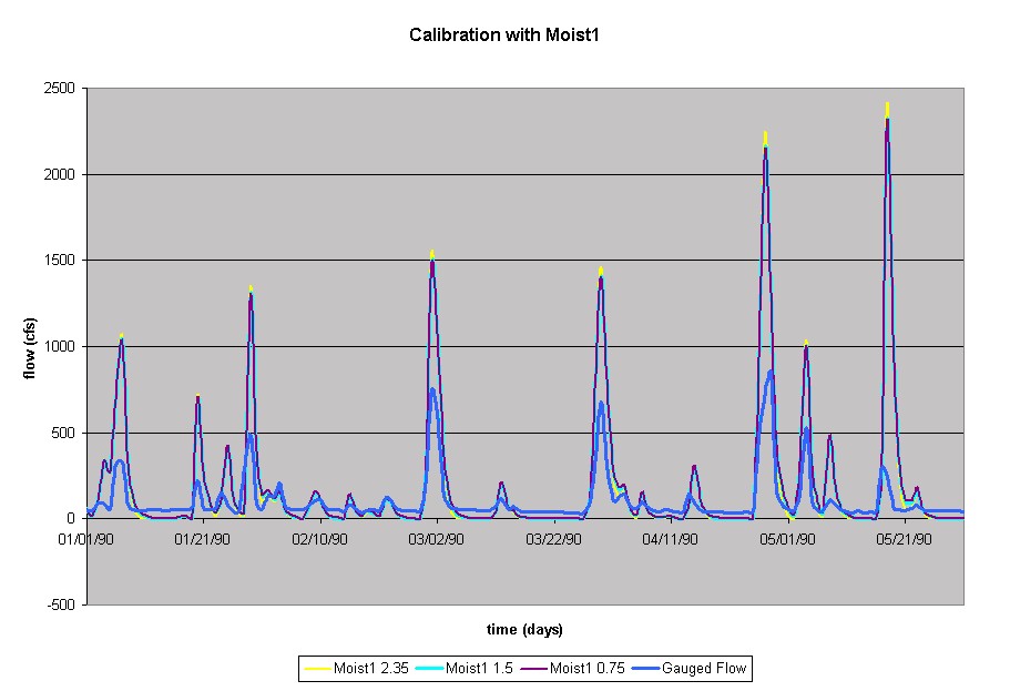
The general tendency of the simulations is that decreasing the Moist1 reduces the peaks above 500 cfs, but increases the peaks below 500 cfs. Also, none of these attempts comes close to successfully replicating the general appearance of the gauged flow. Additional trials were run with more combinations, such as removing 35 cfs as return flow, reducing the Moist1 value further to 0.5 and 0.0, changing to Random Seed A and increasing the abstr1 value to 0.3. The modeled flow continued to look very similar to the simulations shown above. One new aspect to the calibration effort involved the TxRR parameter ranges. When studying the results of a trial using Random Seed A, Moist1 of 0.0, abstr1 of 0.3 and removing a return flow of 35 cfs, a few of the parameters were converging on the minimum value allowed in the input screen ranges. In order to eliminate that as a factor in the fitting process, the parameters A(n) Amp and A (winter) were changed to a minimum range value of 0.0 as opposed to 0.001. This resulted in a slightly better fit, but still too high. Eventually in the trials, the parameter WB1 was also changed to a minimum range value of 0.0. However, all these changes still yielded results shown in the figure above in which the peaks are drastically too high.
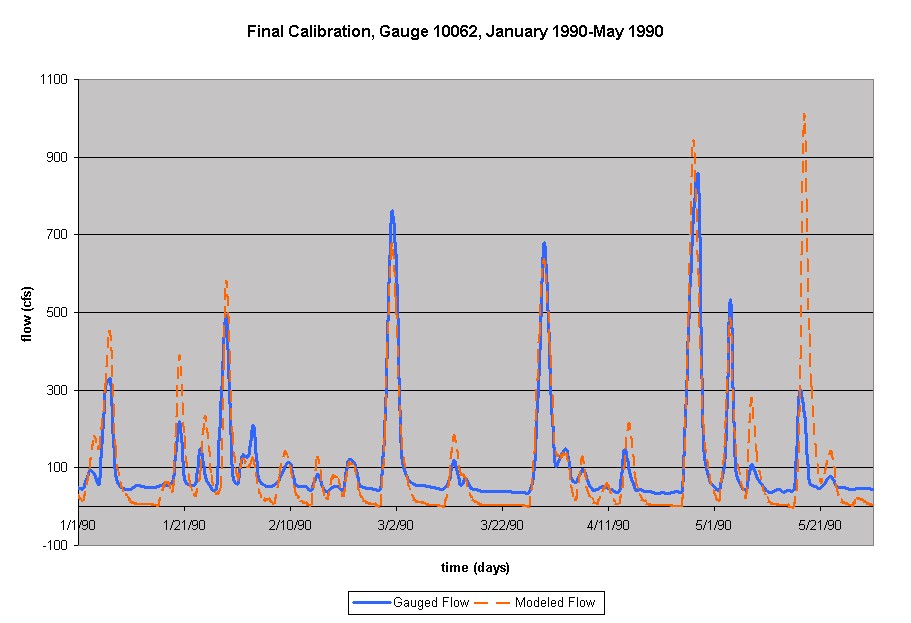
As a "crazy" idea in a desperate attempt to lower the peak flows, the drainage area was decreased from 63.0 sq mi, the value obtained from the USGS, to 50 sq mi. This was done based on the assumption that if there was overall too much runoff from the watershed, less area receiving rain would generate less runoff. This "crazy" idea worked! Although this seemed to be against the "rules" in which the drainage area should be constant and unavailable to be varied during calibration, this unconventional modification had the greatest impact on the simulated flow. When the drainage area was further decreased to 40 cfs, with a Moist1 of 0.0, abstr1 of 0.2 and the A(n) Amp, A(winter), and WB1 minimized to zero, the modeled flow was much better, with the flow generally still too high, but even too low in some places. A trial and error process begin in which it was desired that the smaller peaks increase while the larger peaks decrease. Therefore, the drainage area was continually reduced while the initial moisture Moist1 was increased. After playing with the numbers a bit, a final fit was found. The following graph shows the final calibrated modeled flow and the input and output parameters.
Input
Parameters:
Output Parameters:
|
 |
These results were very confusing, for two main reasons. First, I have trouble with the idea that the drainage area is a variable parameter. However, I can justify this in thinking that the rainfall at the gauging station being used for calibration is not necessarily falling, at that intensity over the entire drainage area. It could be falling over a much smaller area, and therefore using a smaller drainage area in calibration is understandable. Second, in comparing both the input and output parameters, they are vastly different for these two situations, separated by about a year and a half. This result leads me to doubt the validity of my objectives in comparing parameters for different gauged watersheds. Nevertheless, I persevered to calibrate the same simulation period for another gauged watershed.
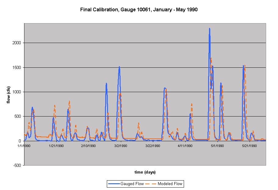
The gauge selected was 10061, with a drainage area of 94.9 sq mi as determined by the USGS. The calibration effort began using all of the default values in the input screen, Moist1 of 2.35, abstr1 of 0.2, no return flow removed, and the USGS drainage area. The result appeared with peaks too high and baseflow too low. To correct for the baseflow issue, the minimum gauged flow, 97 cfs, was removed when prompted. This result was better with the baseflow, but missed the smaller peaks by underestimating and the larger peaks by overestimating. Facing the same problem as the last calibration for gage 10062, the immediate initiative took a turn towards decreasing the drainage area. Again, the drainage area was decreased while the Moist1 was increased. Continual trials led to the Max A(n) difference value increasing to 0.5. Eventually, the final run was found with the best fit, as seen below.
Input
Parameters:
Output Parameters:
|
 |
The results for the two simulations from January - May 1990 and the simulation from December 1991 - June 1992 for gauge 10062 are shown below. As can be seen, the parameters vary greatly over the three models. A few interesting results can be seen: for the storm period modeled for both gauges, the drainage area used to calibrate the model is around 65% of the actual drainage area calculated from the USGS. Also, GammaA, relating to the number of reservoirs to accurately model the hydrographs vary across three orders of magnitude between the calibrations. And, the maximum soil moisture varies across four orders of magnitude as well; most noticeably, for the two calibrations of gauge 10062, it varies across two orders of magnitude. Considering that this relates to the Curve Number of the site, which does not vary, this result is fairly intriguing. All of the parameters can be seen in the following table.
| Parameter | 10061 | 10062 | 10062 (Dec. 91 - June 92) |
| Return Flow Removal | 97 | 0 | 40 |
| Moist1 | 6.0 | 3.0 | 4.0 |
| Drainage Area | 30 | 25 | 63 |
| abstr1 | 0.2 | 0.2 | 0.2 |
| USGS Drainage Area | 94.9 | 63 | 63 |
| D.A. % Difference | -68.39% | -60.32% | 0.00% |
| ibaseflow | 2.0000 | 2.0000 | 2.0000 |
| A phase | 66.2231 | 2.6419 | 0.0000 |
| A Max Difference | 0.5000 | 0.1468 | 0.0537 |
| A(winter) | 0.3000 | 0.0294 | 0.0384 |
| A(1) | 0.7576 | 0.0361 | 0.0384 |
| A(2) | 0.7941 | 0.0738 | 0.0523 |
| A(3) | 0.7971 | 0.1085 | 0.0653 |
| A(4) | 0.7661 | 0.1378 | 0.0764 |
| A(5) | 0.7034 | 0.1597 | 0.0849 |
| A(6) | 0.6131 | 0.1727 | 0.0903 |
| A(7) | 0.5016 | 0.1760 | 0.0921 |
| A(8) | 0.3763 | 0.1692 | 0.0903 |
| A(9) | 0.3542 | 0.1529 | 0.0849 |
| A(10) | 0.4810 | 0.1282 | 0.0764 |
| A(11) | 0.5955 | 0.0968 | 0.0653 |
| A(12) | 0.6898 | 0.0608 | 0.0523 |
| SMMAX | 0.0010 | 0.0127 | 1.4919 |
| RECES | 0.9899 | 0.9894 | 0.9600 |
| WB | 0.0010 | 0.0009 | 0.0024 |
| QB1 | 0.1135 | 0.0078 | 0.0000 |
| GammaA | 3.640822 | 0.501918 | 0.010000 |
| GammaB | 0.024436 | 0.127947 | 0.148454 |
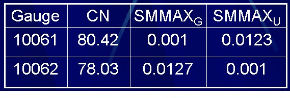
In attempting to use the model for its intended purpose, modeling ungaged watersheds, I employed the relationship between gaged and ungaged watersheds for the TxRR model: SMMAXU = (CNG/CNU) * SMMAXG as if one watershed was gauged and the other wasn't, and compared the results. The Curve Numbers were calculated by the Water Availability Modeling (WAM) project at CRWR. The following table shows the CNs, SMMAX values for the watershed from the gaged calibration and the SMMAX value for the watershed as if it were ungaged, from the watershed relationship. These numbers are vastly different, by an order of magnitude, from their calculated, calibrated values. The TxRR model was then run for the two watersheds using their ungaged SSMAX's in the range of parameters and varying the Moist1 and Drainage Area to observe the results.
When considering the 10062 watershed to be "ungaged", the default input values did not yield a satisfactory result. The default values used were Moist1=2.35, abstr1=0.2 and the drainage area as 63.0, as reported by the USGS. The peaks were again far higher than the actual runoff. When using the drainage area from the calibration and other default values, the modeled flow more closely replicates the recorded flow. The following graph displays the differences and the parameters used for each trial.
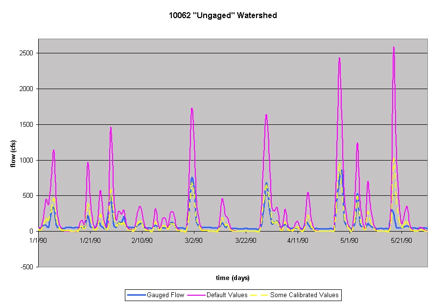
Default Values: Moist1=2.35, Dr. Area=63, abstr1=0.2, no return flow
Some Calibrated Values: Moist1=2.35, Dr. Area=25, abstr1=0.2, no return flow
Similar results were seen when treating the 10061 watershed as "ungaged". Combinations of both the default and calibrated values of the parameters and return flow were attempted. The trial in which no return flow was removed overestimated the baseflow. So again, the return flow was removed at the calibrated amount of 97 cfs, the minimum recorded by the gauge. The graph below shows the results for the "ungauged" trials and the values used for the attempts.
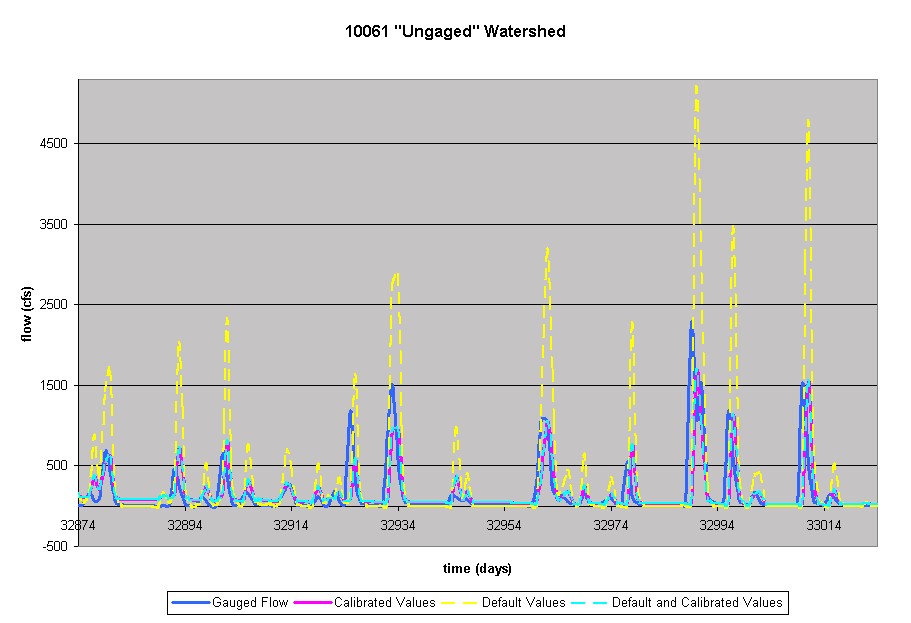
Calibrated Values: Dr. Area=30, Moist1=6.0, remove 97 cfs return flow
Default Values: Dr. Area=94.9, Moist1=2.35, remove 97 cfs return flow
Default and Calibrated Values: Dr. Area=30, Moist1=2.35, remove 97 cfs return flow
The peaks are noticeably too high using the USGS gauge area and fall into place more appropriately using the calibrated drainage area. Additionally, the trials using "Calibrated Values" and "Default and Calibrated Values" are virtually the same, leading to the conclusion that the Moist1 parameter is not that effective in calibrating the flow.
These results are upsetting in that the user would not have a hydrograph to compare the TxRR generated results with for an ungaged watershed. Therefore, the output flow would be greatly overestimated in any subsequent calculations as a result of not reducing the drainage area. By observing the trend seen in the graphs above, only when the calibrated drainage area is used does the TxRR more closely replicate the gauged flow.
In contemplating the reasoning behind better results with a decreased drainage area, the amount of precipitation recorded was called into question. One possibility considered was that the gauge recorded more precipitation than fell over the entire drainage area. To evaluate this option, annual precipitation values in inches were obtained from the WAM final products. The following table shows the amount of precipitation that falls on the gage vs. the amount that falls on the watershed, and the percent difference between them. To compare this percent difference, the difference between the reported and reduced drainage are is also noted.
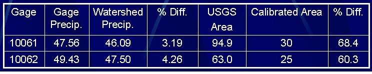
The average difference between the two precipitation values is approximately 4%. These differences do not account for the approximate 65% reduction in drainage area necessary to calibrate the modeled flow. Thus, the rationale behind the drainage area discrepancy is still unknown.
From using TxRR for the Buffalo Bayou Tidal watershed near Houston, many conclusions were determined. First, model calibration is truly an art form, in which the basic hydrologic beliefs must be abandoned and the modeler must "think outside the box". In dealing with the model, a sensitivity analysis of the parameters indicates that the drainage area is the only parameter that leads to any significant change. Ironically, this is the only parameter the user would assume would remain constant throughout the calibration effort. The Moist1 parameter has a small effect, while the abstr1 parameter was held at 0.2, the accepted SCS value. The genetic algorithm parameters of population size and number of children hardly influenced the model outcome and increased the processing time, and were held at the default values. The Random Seed does have an effect on the simulated outflow, but using the default Random Seed A generally provided the best solution in most of the cases.
The TxRR parameters are all calculated by the program and are not user specified. However, the user must compare the final optimized values to the input ranges. On several occasions, the range was modified because the model converged on a maximum or minimum value. While the results after widening the range did not drastically improve, the new optimized values did reflect the change. The last of the input variables, the simulation period, does influence the outcome, in an intuitive fashion. Using a smaller simulation period results in a better initial optimized solution. The user should consider what time frame they are considering when using this model, and use the shorted period possible.
As far as the user-friendliness of TxRR, improvements have been made by Venkatesh Merwade in streamlining the procedures on inputting the data, running the program, and viewing the output. These improvements made the TxRR program much easier to work with, as opposed to the former manner of opening files at a time and calling Fortran routines from DOS. Because TxRR is used mainly by a few employees at the TWDB who actually developed the model, not much documentation exists on the parameters, why default values were chosen, and what some of the parameters actually are. This leads to the user not being able to change much in the model for fear of disrupting another process or altering a physical property to outside an acceptable limit.
Lastly, the usefulness of this model appears to depend significantly on the accuracy of the rainfall and runoff gauged data, and possibly the terrain. As seen in the comparison of results, changing the drainage area is the only modification that made any real impact on the modeled outcome. However, the precipitation data from WAM does not support the theory that this step is justifiable because the entire watershed receives approximately (on the order of less than 5% difference) the same amount of rainfall as the actual gauge itself. Therefore, the rainfall gauge data and the runoff gauge data do not coincide in quantity. A possible explanation relates to the concept of an effect drainage area which can easily apply to such a flat area. When the surface does not have a significant gradient to transport flow over the landscape, a great deal of the watershed surface may just retain the ponded water. There may not enough slope to drive the runoff. Therefore, at certain times, only a certain percentage of the actual watershed may actually contribute to the flow in a stream. This concept has been referred to as a variable source area in hydrologic literature. A variable source area may be caused by variations in the runoff processes (Hortonian overland flow, saturated overland flow, and throughflow) over time and space, specifically during different seasons and during the actual storm event (Pilgrim & Cordery, 1999). This concept's application to flat areas are further reinforced when considering the low surface flow velocity over a flat landscape. In fact, literature states that the source area may be 10% of the entire watershed during a humid well vegetated area (Chow et al., 1988). While those characteristics may not pertain to the Buffalo Bayou watershed, the same principle applies. The relationship evidenced by this research proposes that the effective percentage for this watershed, for the storm period of January - May 1990, may be on the order of 65%.
REFERENCES AND ACKNOWLEDGMENTS
Many people assisted me with this work and provided documentation, aid, data and insight. They are:
|
Venkatesh Merwade, Center for Research in Water Resources |
|
|
Barney Austin, Texas Water Development Board |
|
|
Melissa Figurski, Center for Research in Water Resources, Water Availability Modeling (WAM) Project |
|
|
Dr. Maidment, Center for Research in Water Resources |
Multiple references were used in researching the foundation of the TxRR model as well as the components of it. The following sources were used:
|
Spatially Distributed Modeling of Storm Runoff and Non-Point Source Pollution Using Geographic Information Systems. Francisco Olivera, David R. Maidment, & Randall J. Charbeneau, 1996. Chapter 4: Methodology. Internet Site: http://civil.ce.utexas.edu/prof/olivera/disstn/chapter4/meth.htm |
|
|
Genetic Algorithms. Marek Obitko, 1998. Internet Site: http://cs.felk.cvut.cz/~xobitko/ga |
|
|
Introduction to Genetic Algorithms. Nick Johnson. Internet Site: http://members.aol.com/DaemonBBS/ai/tut/intro.html |
|
| User's Manual for The TWDB's Rainfall-Runoff Model. Junji Matsumoto, PhD. PE. Texas Water Development Board. | |
| Developing a GIS-TxRR Model. Jerome Perales, Richard Gu, & David R. Maidment. Center for Research in Water Resources. | |
| Geographical Database Development for the TxRR Surface Water Model. Richard Gu. | |
| Chapter 9: Flood Runoff. David H. Pilgrim & Ian Cordery, 1999. Handbook of Hydrology, David R. Maidment. | |
| Applied Hydrology. V.T. Chow, D.R. Maidment, & L.W. Mays, 1988. Chapter 5: Surface Water. |