The National Hydrography Dataset and Network Capabilities in Arc GIS 8

This exercise will introduce the user to hydrography data, specifically from the National Hydrography Dataset. The user will learn to symbolize and differentiate between the feature and reach data layers. The attributes accompanying the hydrography data will also be discussed.

The new network capabilities in ArcGIS 8.0 will then be utilized. The user will:

Additional ArcGIS functionality will be explained and incorporated into the exercise.

The study area selected for this exercise is HUC #12040204, West Galveston Bay. This area is located on the Southeast coast of Texas near Houston.

To carry out this exercise, you need to have a computer which runs ArcInfo 8.0 (with ArcMap and ArcCatalog). In order to download the National Hydrography Dataset data, you will need internet access. However, the data will also be provided in the accompanying zip file, Networks.zip, which you can get from this link. For UT Austin students, the files are located on the LRC NT network in the directory class\maidment\giswr\networks\.

The data files used in the exercise consist of ArcInfo coverages. All of the data being used is in the Geographic projection. The following files are required for this exercise and are stored in the file Networks.zip:

The National Hydrography Dataset (NHD) is an substantial set of digital data and contains information about the surface water drainage network. The data consists of naturally occurring and constructed bodies of water, natural and artificial paths which water flows through, and related hydrographic entities. The NHD is distributed by the United States Geological Survey (USGS) and is available to the public for download. An optional part of this exercise is manually downloading the data from the website, which is useful for future reference.

The NHD is available at the website http://nhd.usgs.gov. Click on the Data tab on the left side of the screen and then click on the first bullet, Obtaining NHD Data. The NHD is organized by Hydrologic Cataloging Unit (HUC). You will see a map of the United States in which you can zoom in and navigate to the HUC of interest. Another option is using the FTP site to obtain the data. The data you will be using is for HUC #12040204. The first method described is downloading the NHD using the map. If you choose to use the FTP site, skip the next three paragraphs to the next method.

Zoom in several times on Eastern Gulf Coast of Texas near the Louisiana border (the divide between green and light green HUCs). Eventually zoom in to where you can differentiate between HUCs and their number.

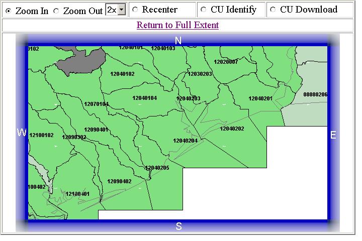
When you can distinguish HUC #12040204 (the third green HUC to the left after the border between green and light green HUCs), change the radial button at the top of the map to CU Download and click on HUC #12040204. Fill out the NHD Download screen information and Continue. Click Yes to the Security Warning and click Download on the Download page.

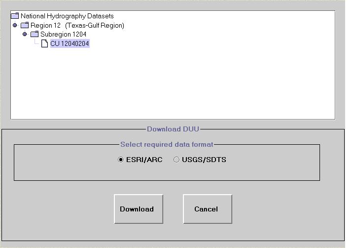
Navigate to the location you want to place the 12040204 file, and click OK to the Successful Download window. You now have the 12040204.tgz file, a compressed folder with the NHD data.

Another way to download the data is to use the FTP site, if the HUC number is known. You want HUC #12040204, and can precede directly to the FTP site without manipulating the map. From the initial window with the map of the United States, click on the FTP link under the map. Scroll down the list to the 12040204.tgz link, click on it, then Save this file to a disk. Navigate to the directory you want to place the data.

Now you have the NHD data for HUC #12040204. If you chose not to download the data from the website, the zip file 12040204.tgz can be found in the Networks.zip file accompanying this exercise.

Unzip the 12040204.tgz file using the Windows utility Winzip. Extract the file to the 12040204 folder. Click Yes to the Winzip window asking if Winzip should decompress 12040204.arc.tar to a temporary folder. In Windows Explorer, navigate to the second 12040204 folder.

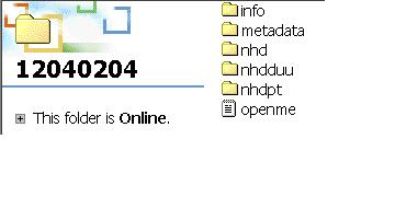
The NHD is organized as three ARC/INFO coverages, many related INFO tables, and text files containing metadata. The nhd coverage contains the line and polygon features. This coverage has line, polygon and node topology, which together is network topology. The nhdpt coverage contains point features related to the hydrography. The third coverage, nhdduu, contains metadata and information about sources and updates of the hydrographical information. The spatial elements of the surface water network are found in the nhd and nhdpt coverages.

Open a new empty map in ArcMap and Add Data. Browse to the second 12040204 folder, then to the nhd folder.

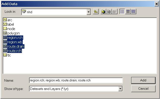
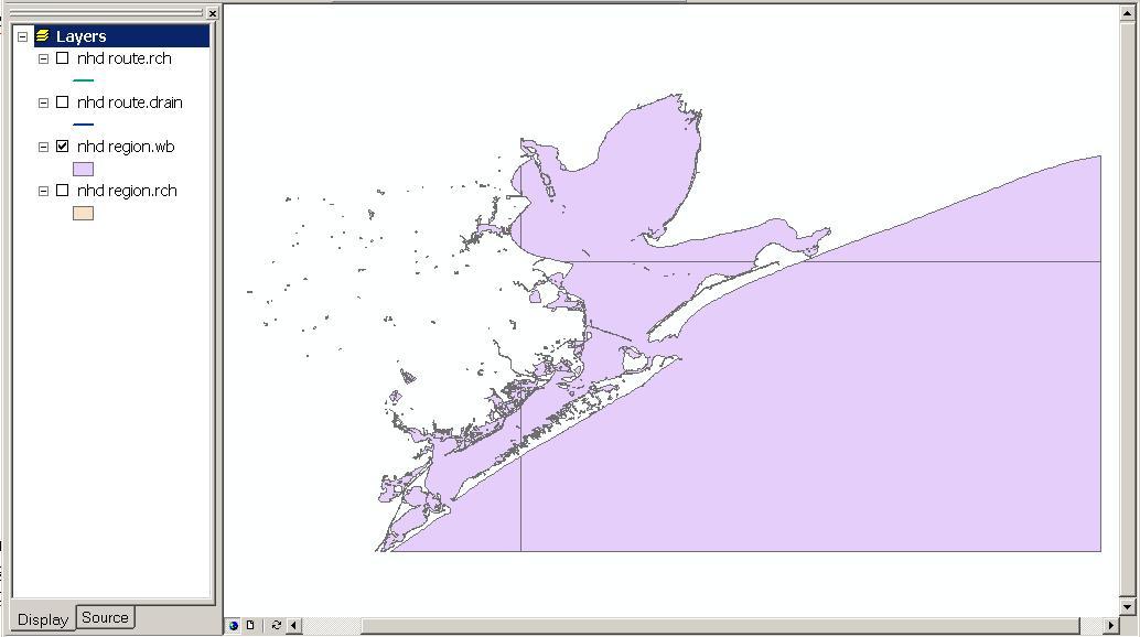
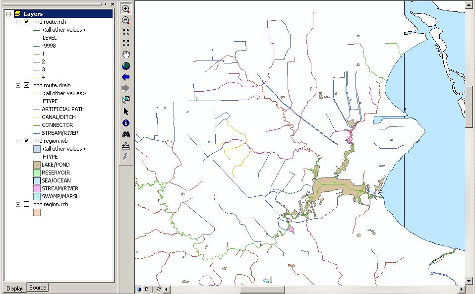
Note the different elements in the nhd coverage. Arcs, nodes, and polygons are the typical spatial elements originally in ArcInfo. The NHD forms groups of arcs or polygons as single entities and labels them as routes or regions, respectively. Add the region.rch, region.wb, route.drain, and route.rch data layers.

Now turn off (remove the check in the box) for all layers except region.wb. This theme contains the areal hydrographic features representing waterbodies. They are organized in "regions" as opposed to individual polygons because one waterbody may be composed of many polygons in the ArcInfo environment. In order to look at the entire waterbody, not just pieces of it, we use the region themes.

The region.wb layer displays many types of waterbody features. These are: Area of Complex Channels, 2-D Canal/Ditch, Estuary (in the next release), Ice Mass, Lake/Pond, Reservoir, Sea/Ocean, Swamp/Marsh, 2-D Stream/River, Playa and Wash. To classify these different types uniquely within the region.wb layer, doubleclick on the nhd region.wb data layer name, or right click on the layer name and go to Properties. Go to the Symbology tab. To symbolize each type of waterbody uniquely, click on Categories and highlight Unique values. From the Value Field dropdown menu, select FTYPE. Then click on Add All Values. This adds all the different values of Ftype present in this data layer to the legend and symbolizes them differently. For each feature class, the Ftype attribute describes what type of feature an element is. The Fcode attribute is a coded value for that type.

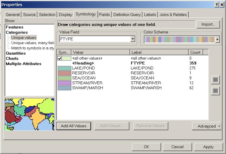
Choose each type of waterbody to look differently. To change all of the Ftype legends at once, change the color ramp from the Color Scheme dropdown menu. You can change the individual types by clicking on the color box next to the type name. ArcMap has preset legend styles contained in the symbology options. These preset styles store different industry's standards of representing certain spatial data. These include waterbodies, transportation ways, signage, etc. Click on the color box of Swamp/Marsh. Scroll down on the Symbol Selector window, and select Swamp.

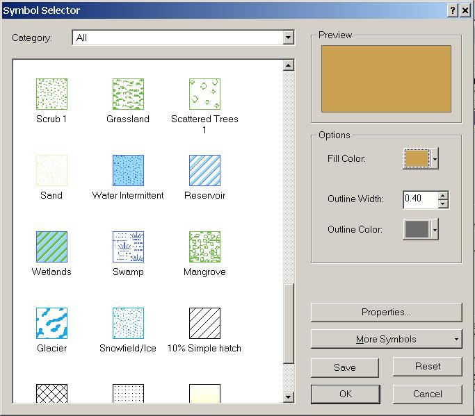
To make the background color of the Swamp filled in and easier to see on the map, click on Properties. On the Picture Fill tab, change the background color to be a color as opposed to white. Leave the foreground color as blue, or change it as you would like. Click OK and click OK to close the Symbol Selector window. Change any additional Waterbody types to look as you would like. Click OK and close the Layer Properties window.

Zoom in on various areas on the map to see the boundaries between lakes, swamps, oceans and streams.

In addition to the Ftype attribute, the region.wb data layer contains other descriptive information. Rightclick on the nhd region.wb data layer and Open Attribute Table. The fields of interest for the region.wb data layer are:

Additional attributes are identifiers. One identifier common to all of the NHD region and route data layers is the COM_ID. The is a unique identifier given to each NHD feature or reach. In this data layer it is called the WB_COM_ID. The COM_ID, or common identifier is a 10 digit number which is distinct for each feature within all of the NHD. It is used as a reference to relate the various data layers as will be seen later in the exercise. An additional attribute, RCH_COM_ID, will be discussed later as well. Close the Attribute Table.

Zoom out to the entire extent and turn on (place a check in the box next to) the route.drain theme. This layer encompasses the entire linear surface water drainage network. The features represented in this layer are: Stream/Rivers, Canal/Ditches, Pipelines, Artificial Paths that run through the waterbodies described earlier, and Connectors. As described above, these linear features are grouped together as routes rather than simple lines because several lines may comprise one route. Symbolize all values uniquely based on Ftype, as you did in the previous section.

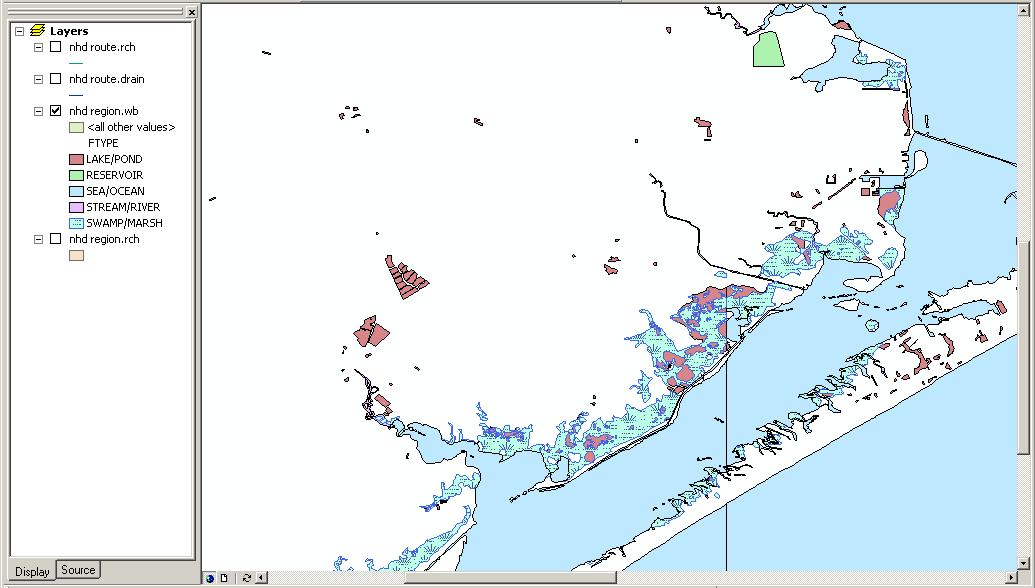
Observe the artificial paths which run through the waterbodies of the region.wb layer. Zoom in on the lake in the upper right corner of the basin.

Notice the artificial paths running through the lake/pond and 2-D stream/river features. Coastlines bordering the sea/ocean are also considered artificial paths. The artificial path immediately changes to a stream/river when it exits the waterbody. These artificial paths represent flow paths where there is realistically no actual channel. Using these artificial paths aids in performing network tasks which you will do later in this exercise. Without the artificial paths and connectors, the network would have breaks at any waterbody features.

Also notice the overwhelming amount of canals versus natural streams in the area. Because this area is so flat and near the coast, the relief does not always determine the direction of flow. Several manmade canals were added to the drainage network.

In addition to the Ftype attribute, the route.drain data layer also contains other descriptive information. Rightclick on the nhd route.drain data layer and Open Attribute Table. The fields of interest for the route.drain data layer are:

Now, zoom back out and turn on the route.rch layer. This is the linear drainage network as well, broken up into different pieces called reaches. A reach is generally the sum of all surface water features with similar hydrologic characteristics. This can be either pieces of stream/rivers, or portions of lake/ponds. There are three types of reaches: transport, coastline, and waterbody. The transport and coastline reaches are found in the route.rch data layer, while the waterbody reaches are found in region.rch data layer which will be studied next. A fourth type of reach, shoreline reach, has not be developed yet. Reaches are used as tools to geocode information about a linear or areal surface water feature because of their identifying attributes.

Transport reaches represent the path of water moving across the drainage network. Coastline reaches represent the coastline of the Atlantic, Pacific, or Artic Ocean, the Great Lakes, the Gulf of Mexico, or the Caribbean Sea. They are used to reference the location of the ocean in respect to the drainage network. Coastline reaches are only composed of artificial paths.

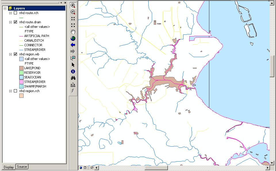
Now you will look at how several features in the route.drain layer can comprise one element in the route.rch layer. Each reach element in route.rch is given a unique identifier, called the Reach Code. The Reach Code is a 14 digit number with two parts: the first eight digits are the Hydrologic Cataloging Unit code for the Unit in which the reach is located, and the second six digits are a unique number assigned to each reach arbitrarily. You will symbolize two of these reaches uniquely to look at their composition. Double-click on the route.rch layer, click on Categories and highlight Unique values. Change the Value Field dropdown menu to RCH_CODE. Click on Add Values... and click Yes to the warning. Highlight 120402000174 and 12040204000948 by holding Control to select the second choice. Click OK. Change these colors to something bright and noticeable. Zoom in to the area containing both these reaches (the bottom left of the screen).

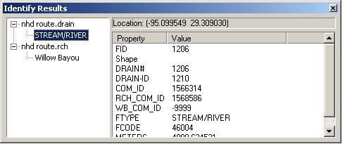
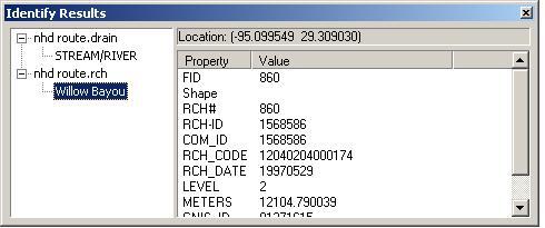
Both of these reaches are composed of multiple drain feature elements. To see the grouping of network elements in one reach, go to the Selection menu and drag down to Set Selectable Layers, check nhd route.drain and uncheck the other layers. Using the Select Features button, click on one of the reaches. Notice how only a portion of the reach becomes highlighted. This is only one of the network elements that make up the one reach. Reach 12040204000174 is made up of three distinct features and reach 12040204000948 is made up of 2 different feature elements. The drain features composing each reach and that corresponding reach are linked together through the RCH_COM_ID in the route.drain layer. In the route.drain layer, the RCH_COM_ID is the COM_ID identifier of the reach which the network element is part. Using the Identify tool, click on the selected portion of the reach. Swith back and forth on the left side menu in the Identify Results box between nhd route.rch (the name of the reach) and route.drain (the type of feature). Note that the COM_ID for Reach 12040201000174 is 1568586 and the RCH_COM_ID for all three drain features that comprise it is also 1568586.

Another important attribute in route.rch is Level. The Level attribute characterizes the stream level of each reach. The level is determined by first identifying the endpoint or sink of the surface water drainage network, and working backwards by the flow relationships. The lowest level (one) is assigned to reaches which flow into the endpoint and to upstream transport reaches which trace the main flow of water back to the head of the stream. The level is then increased by one for reaches which terminate at the main flow path, i.e. reaches which are tributaries to the main flow path. This procedure continues to assign a level attribute to all reaches. If a reach has a level of -9998, the level for that reach is currently undefined. Either the reach is isolated and not connected to the network, or the level is not yet determined. Most of the canals in this area of of level -9998 since their complex nature does not allow a flow direction to be defined. Additionally, the coastline reaches are also -9998 level because they do not have a specified flow direction.

Go to the Selection menu and Clear Selected Features. Go to the Symbology tab of the nhd route.rch Properties and change the Value Field to LEVEL. Add all the values and choose a Color Scheme that displays the levels clearly and vibrantly. Zoom to Full Extent (the globe button on the Tools toolbar) and then again zoom into the area by the lake. Notice all four level values as well as the level value -9998.

Go to the Selection Menu and go to Set Selectable Layers. Change the selectable layer from nhd route.drain to nhd route.rch. Using the Select Features tool on the Tools toolbar, select the lines in the lake. Notice how all the line features within the lake are selected as a single reach. Because all these internal drain elements contain the same hydrologic characteristics, they are considered one reach. Select a few of the upstream level one segments flowing into the lake. Open the attribute table of nhd route.rch and click Selected for Show ... Records.

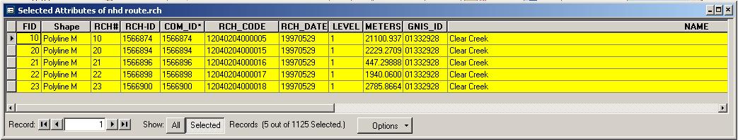
Each of the selected streams has a level of one, which is the main flow path from the bordering bay. The nhd route.rch data layer also has the attributes of GNIS_ID and NAME as in the region.wb data layer. All of these reaches make up a part of Clear Creek, which is referenced by the GNIS as 01332928. An additional attribute of note of the route.rch layer is the RCH_DATE. This the date that the Reach Code (RCH_CODE) was first assigned. The additional attributes will be discussed later. Clear the selected features.

The final layer you will look at is the waterbody reach data layer. Turn on the nhd region.rch layer, and highlight its name. Click and drag the data layer to above the region.wb data layer. These polygons are regions which represent waterbody reaches. These regions are composed of one or more regions found in region.wb. Just as transport and coastline reaches allow for information to be linked to the linear network features, waterbody reaches allow for information to be attached to areal features. In this first release of the NHD, waterbody reaches are only defined for lake/pond features in region.wb. For these lake/pond areas, it is possible for both a transport and waterbody reach to be defined; the transport reach represents the artificial path of flow through the lake while the waterbody reach describes the area.

Go to the Symbology tab of the Properties of region.rch and symbolize the data layer by RCH_CODE. Click on the minus sign next to the region.rch layer name in the Display Table of Contents to shorten the legend list. The attributes of nhd region.rch are:

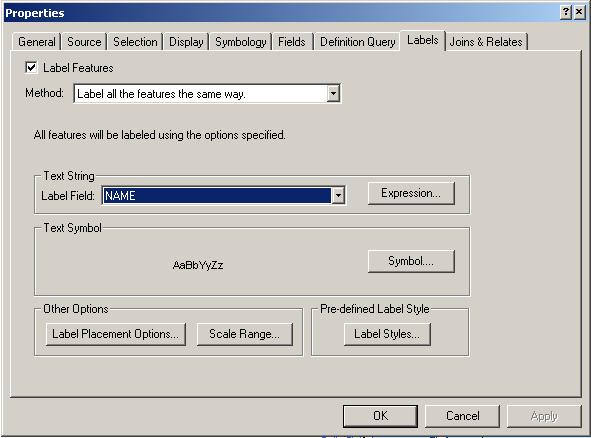
It is possible to view those waterbodies that have names assigned by the Geographic Naming Information System. Right-click on the region.rch layer name. Go Properties, then go to the Labels tab. Change the dropdown Label Field: menu to NAME. Click OK.

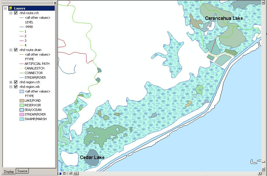
Right-click again on the region.rch data layer. Go to the Label Features option. Now all the waterbody reach regions that have names assigned by the Geographic Naming Information System are shown. Zoom in on Carancahua Lake and Cedar Lake. You can change the appearance of the labels from the Labels tab of the Properties, and make the text larger and darker. The relationship between the route.drain and route.rch data layers also exist between the region.wb and region.rch data layers through the RCH_COM_ID. Check the different attributes of COM_ID and RCH_COM_ID using the Identify tool for Caranchahua and Cedar Lakes.

In addition to the layers described above, the National Hydrography Dataset contains hydrographic features which do not necessarily play a role in the network. These features are known as Landmarks and are found in the NHD as route.lm and region.lm in the nhd coverage folder for lines and areas and as the nhdpt coverage for points.

The attributes of these landmark layers are shown in the table below. The attributes are all found in other data layers and their description can be found earlier in this exercise.

Region.lm

Route.lm

Nhdpt

COM_ID

FTYPE

FCODE

ELEV

STAGE

SQ_KM

GNIS_ID

NAME

COM_ID

FTYPE

FCODE

METERS

GNIS_ID

NAME

COM_ID

FTYPE

FCODE

GNIS_ID

NAME

For the FTYPE for each data layer, the options are very diverse and very encompassing of any type of hydrologic landmark feature. The types of feature for each data layer are listed below:

Region.lm

Route.lm

Nhdpt

Area to Be Submerged

Bay/Inlet

Bridge (2-D)

Dam/Weir (2-D)

Foreshore

Hazard Zone

Inundation Area

Lock Chamber (2-D)

Special Use Zone

Submerged Stream

Spillway

Rapids (2-D)

Bridge (1-D)

Dam/Weir (1-D)

Gate (1-D)

Lock Chamber (1-D)

Nonearthen Shore

Rapids (1-D)

Reef

Sounding Datum Line

Special Use Zone Limit

Tunnel

Wall

Waterfall (1-D)

Fumarole

Gaging Station

Gate (0-D)

Geyser

Lock Chamber (0-D)

Mudpot

Rapids (0-D)

Rock

Spring/Seep

Waterfall (0-D)

Well

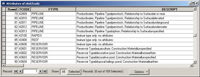
Different features may be represented in multiple dimensions, such as Rapids, which can be present in all three data layers. Many of these types of features have multiple subtypes which is characterized in the FCODE attribute. The first three digits of the FCODE indicate the feature type and the last two digits describe the distinct characteristics. To look at the different types of characteristics associated with each FTYPE and to determine the meaning of the FCODE, you will load a table that comes with the NHD data. Click on the Add Data button and navigate up to the root 12040204 folder and add nhd.fcode.

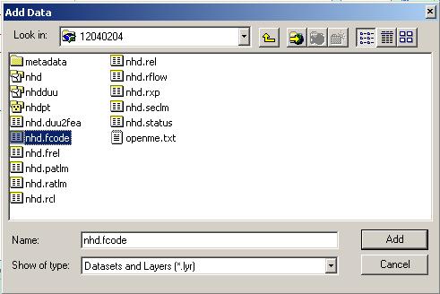
The Table of Contents should have switched to the Source tab with the table nhd.fcode at the bottom. Right-click on nhd.fcode and go to Open. The table lists the various FCODE values, the FTYPE text that accompanies that FCODE, and the description of the FCODE which highlights the differences between them. Notice how many different subtypes of each one feature type that exists.

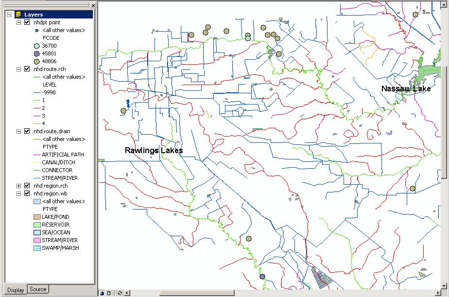
There are no linear or areal landmark features for the area studied in this exercise. However, there are landmark points. Add the data layer nhdpt from the folder 12040204. Right-click on the nhdpt point data layer and Zoom to Layer. Symbolize the nhdpt layer uniquely based on FCODE. Look up what each FCODE means in the nhd.fcode table to determine what each type of point is.

You have now thoroughly inspected the feature data from the National Hydrography Dataset. Save this map and exit ArcMap. Additional information about the NHD can be found at http://nhd.usgs.gov/techref.html in the documents:

You will now use the route.rch data layer to perform network analysis functions available in ArcGIS 8.0.

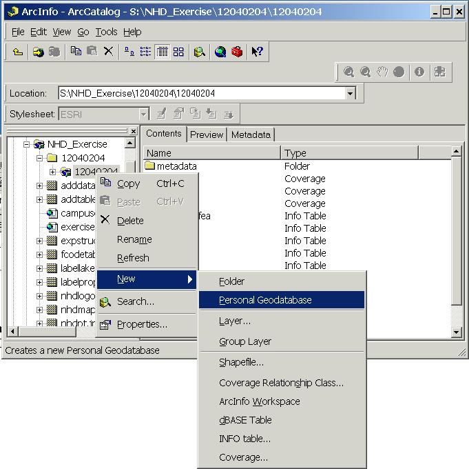
Within the new functionality of ArcGIS 8.0, the ability to trace along networks based on flow directions and relationships is central. In order to use these functions, a geometric network must be built. Open ArcCatalog and navigate to the 12040204 folder.

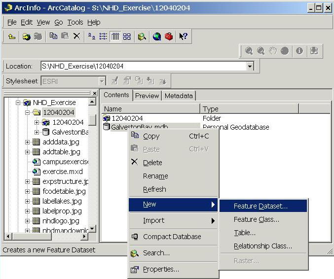
Right-click on the 12040204 folder in the Table of Contents on the left. Drag down to New, then drag over to Personal Geodatabase.

Name the geodatabase GalvestonBay. Right-click on GalvestonBay.mdb and drag down to New and then to Feature Dataset....

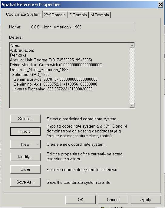
Enter the Name: for the Feature Dataset as West_Galveston_Bay. Click Edit.. for the Spatial Reference and click on Import... Navigate to the 12040204 folder/nhd/route.rch. This sets the extent for the feature dataset to the same as the extent for the route.rch data layer. Click OK.

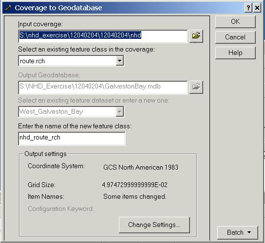
At this point, you want to enter data layers directly into the feature dataset West_Galveston_Bay. Right-click on the feature dataset West_Galveston_Bay and drag down to Import and Coverage to Geodatabase. For the Input coverage:, browse to the 12040204/nhd/route.rch data layer. Click OK. The software then converts the coverage into data within the feature dataset.

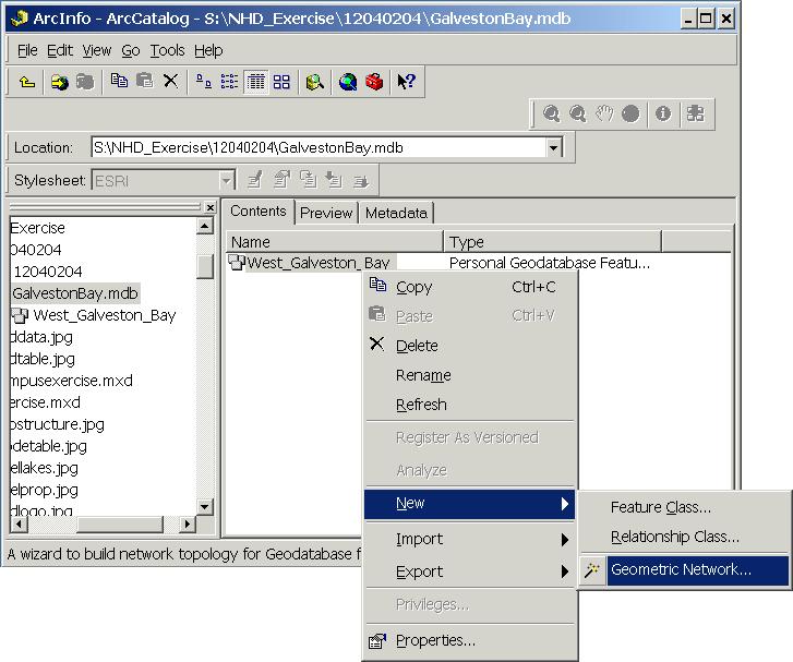
Similarlly, add the Sinks coverage from the Networks.zip file to the West_Galveston_Bay feature dataset by again importing from Coverage to Geodatabase in ArcCatalog. Choose teh points feature class from the Sinks coverage. From the West_Galveston_Bay feature dataset, right-click and drag down to New and to Geometric Network...

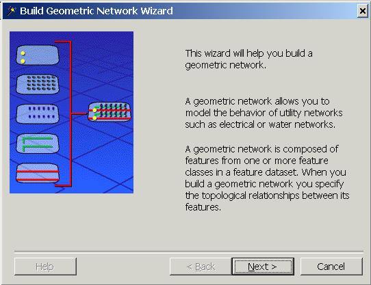
This launches a Build Geometric Network Wizard to help you create a network from a feature class in a feature dataset. Click Next.

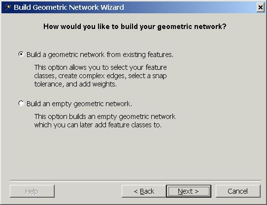
Because you have the route.rch data layer as the arcs which you want to use as your network and Sinks to determine flow direction, you want to Build a geometric network from existing features. Make sure this radial button is highlighted and click Next.

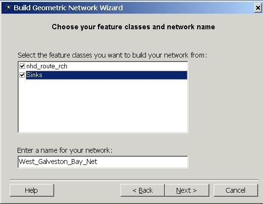
The next screen determines which existing features should be incorporated in the network. Because you have entered two feature classes into the feature dataset, they are listed as defaults. Check both nhd_route_rch and Sinks and enter the name West_Galveston_Bay_Net. Click Next. Click OK to the ArcCatalog Warning about the "Enabled" field.

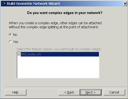
For Do you want complex edges in your network?, the nature of the data model that we are working with only supports relationships with simple edges. Therefore, make sure the radial button for No is highlighted and click Next.

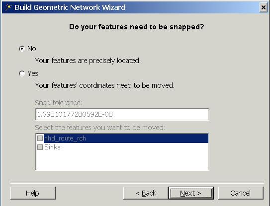
The sinks accompanying the network were selected directly from junctions on the nhd_route_rch data layer; therefore they fall exactly on the network and do not need to be snapped. Highlight the radial button No for Do your features need to be snapped? and click Next.

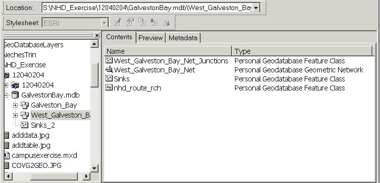
The file Sinks contains the sinks for this coastal area of West Galveston Bay. Click Yes for the network to contain sinks and make sure that Sinks is checked. Click Next. If there is a Warning, click OK. The network you are working with has no weights assigned to it, so make sure the radial button has No highlighted and click Next. A summary is then displayed of the input information. Check over this information to ensure it is correct, and click Finish. The elements of the feature classes are then converted to have network topology. In ArcCatalog, look in the feature dataset West_Galveston_Bay. A new icon and new feature classes are added, the West_Galveston_Bay_Net network and its accompanying West_Galveston_Bay_Net_Junctions which are automatically created when the feature classes are converted to have topology. Close ArcCatalog. Now you want to look at the network within ArcMap to use the network functionality.

Open your ArcMap exercise. You will now add a new data frame, the equivalent of adding a new View in ArcView. On the bottom of the viewing screen, there are three buttons. The first shows the data frame (view in ArcView) you are working with, the second shows the layout, and the third refreshes the display. Switch to the layout view by clicking on the second button. Click on the Insert menu and drag down to Data Frame. Now switch back to the data frame displays by clicking on the first button. Scroll down to the bottom of the left Table of Contents to see the New Data Frame. To change the name, right click on the New Data Frame and go to Properties. Click on the General tab and change the Name: to Network.

Click on Add Data and navigate to the West_Galveston_Bay feature dataset, and highlight the West_Galveston_Bay_Net and add it to the Network data frame. The data layers nhd_route_rch, Sinks, and West_Galveston_Bay_Net_Junctions are added.

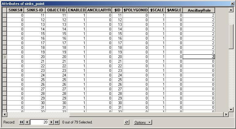
To generate the flow direction along the network, the sinks must have an Ancillary Role value of 2, indicating a sink. The other available Ancillary Role values are 0 for None and 1 for Source. You will now assign the Ancillary Role value of Sink to the points in the Sinks feature class. Add the Editor toolbar by going to the View menu, Toolbars, and make sure there is a check next to Editor. On the Editor Toolbar, click on Editor and drag to Start Editing. Right-click on Sinks and Open Attribute Table. Notice that the points currently have a AncillaryRole of 0. Click in the AncillaryRole box for each point and change the value to 2. Do this for all of the points in the attribute table.

Close the attribute table and click again on Editor. Drag to Save Edits. Now the flow direction for the network can be determined. From the View menu, go to Toolbars and check the Utility Network Analyst toolbar.

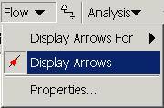
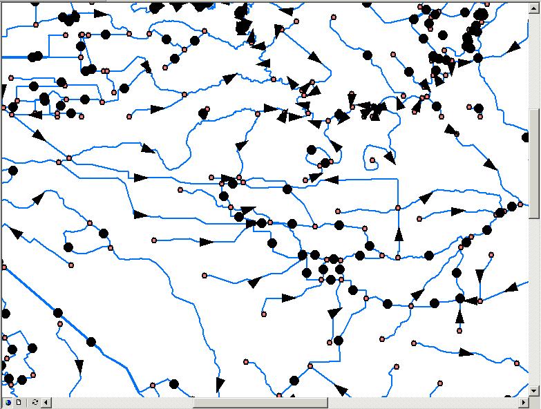
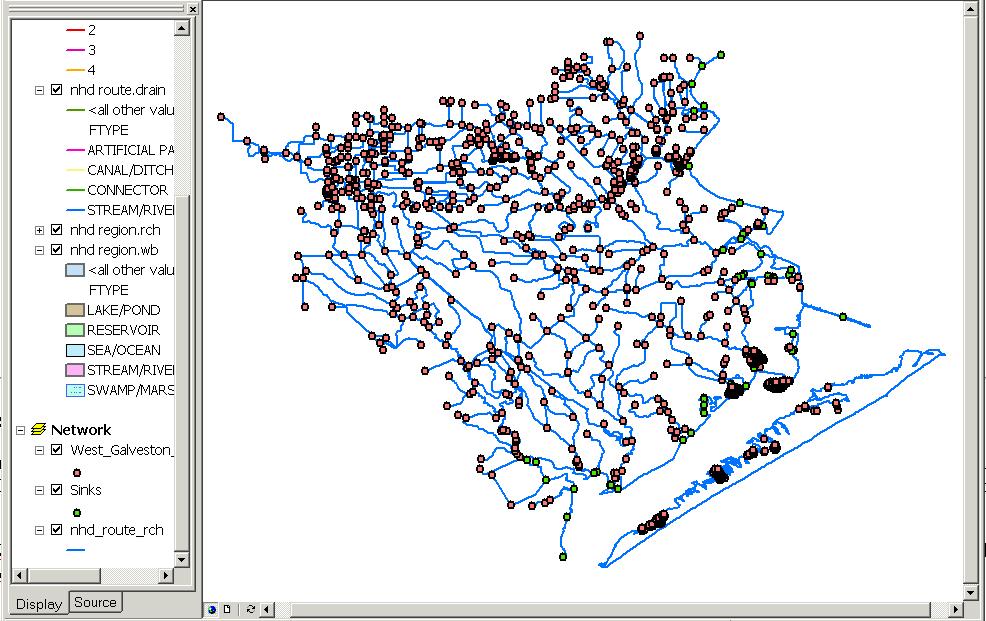
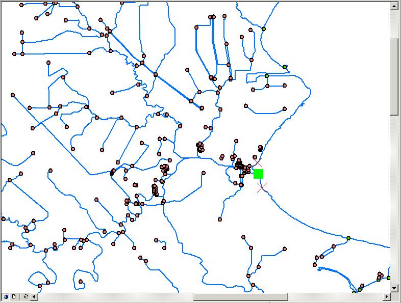
Between Flow and Analysis is an icon with sets flow direction. Click this icon, then click on the Flow dropdown menu and go to Display Arrows. The arrows may not all appear and only some dark circles may appear. The software is still not foolproof when displaying the arrows. If you have a problem, try turning on off display arrows, and that may work. If not, the picture below shows how the arrows should appear.

Each reach in the network has an arrow or a circular "blob" on it to indicate the flow direction along that reach. A circular "blob" indicates that the flow direction is indeterminate along that reach. This is caused by looping in the network, in which the path that the water would flow cannot be chosen. Zoom into an area to see the arrows and how the flow progresses down the network. The area studied in this exercise has many indeterminate flow paths because it is along the coast. Coastal areas generally have more looping in the network, leading to undetermined flow direction.

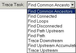
Because it takes longer for the screen to redraw with the arrows, turn them off by going back to the Flow dropdown menu and click again on Display Arrows. Now that the flow direction has been determined, it is possible to perform traces on the network to determine topology relationships between reaches. The Trace Task menu lists the options that are available:

Find Common Ancestors - Find the common features that are upstream of a set of points in the network
Find Connected - Find all features connected to a given point in the network
Find Loops - Find loops that result in multiple paths between points in the network
Find Path - Find a path between two points in the network.
Trace Upstream - Find all network elements that lie upstream of a given point in the network
Trace Downstream - Find all network elements that lie downstream of a given point in the network

We first want to set a few general parameters before tracing. Click on the Analysis dropdown menu and go to Options... On the General tab, click Directed trace tasks include edges with indeterminate and uninitialized flow. This means that the tracing tasks will go through those reaches with indeterminate flow direction and keep tracing instead of stopping when the trace meets a reach with undefined flow. With this option, tracing along loops and the coastline is possible. Click Apply. On the Results tab, change the Results format to Selection. Now the trace results will be shown immediately as a selection which can then be exported to a feature class if desired. Click OK.

Tracing tasks are defined by first placing flags and barriers along the network to indicate where the trace should start and stop respectively. The icon after the Analysis menu places the flags and barriers. There are four options:

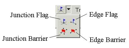
Junction flags and barriers are placed at junctions, while edge flags and barriers are placed along edges. When using an edge flag or barrier, the trace either begins or ends and includes that entire edge, as opposed to only a portion of the edge.

The first trace you will perform is Tracing Upstream. Place a Junction Flag at the sink with ObjectID (FID) 6 (at the upper right side of the area, the 5th sink in, use the Identify tool to find it). Place Edge Barriers on the reaches on either side of the Junction Flag. Be sure to place the edge barriers a significant distance from the junction. The purpose of these barriers is to stop flow along these reaches because we do not want them selected. Because they have indeterminate flow and we turned on the option of tracing along undefined flow paths, a trace would include these reaches; however, the barriers should stop this.

To perform the trace function, you must set the Trace Task from the drop down menu as Trace Upstream and then click the Solve icon next to the menu. The solution appears as a selection. From the Selection menu, drag down to Zoom to Selected Features to see the reaches upstream from Sink 6.

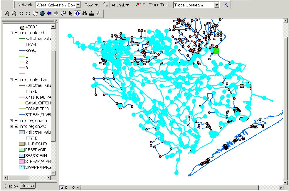
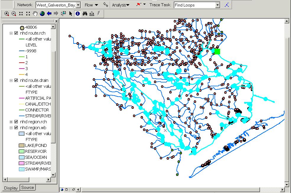
You can see that most of the reaches were selected as the solution to the trace upstream. This does not appear correct; however, it is for the task defined. Again, because we chose to trace along reaches with undefined flow direction, the vast looping in the area wound up connecting most of the reaches to the junction in question. We can see the loops in the area by using the Find Loops trace tasks. We will take off the barriers from the network to find all the loops. From the Analysis menu, go to Clear Barriers. From the Selection menu, chose to Clear Selected Features. Now change the trace task to Find Loops and click the Solve icon. This selection shows the loops from that one junction. Now extrapolate this results to the whole study area, and you can realize how many of the reaches are connected by some sort of loop. This explains the Trace Upstream results.

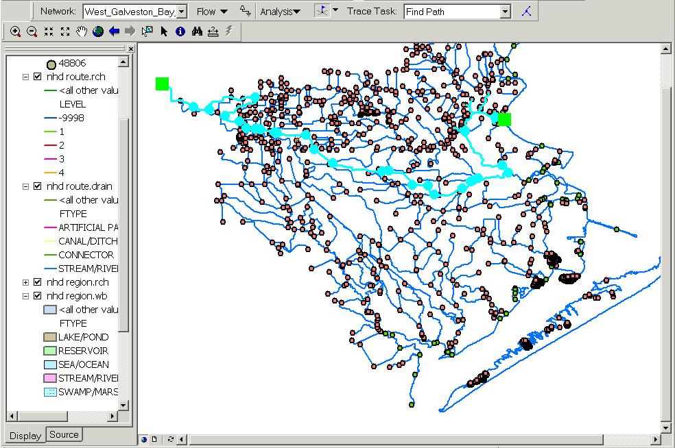
A trace that will yield cleaner results is the Find Path task. You will find the path between Sink 6 and the apparent headwater junction, at the top left of the area (see the below picture for the location). Clear the selected features. Place another Junction Flag at headwater junction. Change the Trace Task to Find Path and click the Solve icon.

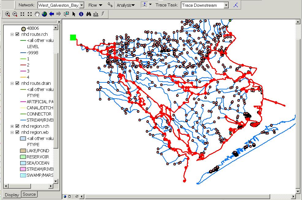
The final trace task you will perform will be a Trace Downstream from that apparent headwater junction. Clear the flags and the selected features. Place a new flag at headwater junction. You will also utilize the other method of returning results in tracing. From the Analysis dropdown menu, go to Options.. and the Results tab. Change the radial button for Results format to Drawings. By returning the results as a drawing, you cannot use the results for anything other than viewing. With the results as a selection, it is possible to convert that selection to a new feature class, or look at the selected features in the attribute table. Change the Trace Task to Trace Downstream and click the Solve icon. The results are similar to the Trace Upstream results because of the looping.

To clear the results as a drawing, go to the Analysis menu and go to Clear Results. Save your ArcMap map. Be creative and try other traces from other junctions. Experiment using barriers on both edges and junctions. When you are finished, close the Edit Session by going to the Editor menu and Stop Editing. Say Yes to saving the edits, and save and close the map document.

You have now finished this exercise. Congratulations! These lessons should assist you in using ArcMap and ArcCatalog as well as provide information about a useful data source.