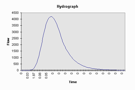
Hydrograph
"Rainfall/Runoff Simulation"
Term Paper- 394K Surface Water Hydrology- Dr David Maidment
December 6, 1996
Hydrograph
The inspiration for my study is my fascination with the ability of humans to describe natural phenomenon with mathematical relationships. When I realized that math could be used in this way, I had a whole new respect and love for math. This semester I became interested in hydrologic simulation models used to simulate rainfall/runoff processes in watersheds. This report will begin with work I did but was unable to complete and then I will describe the work that I was able to do with the time I had remaining.
HECHMS Watershed Model
The goal of my study was to learn more about hydrologic simulation models.
The watershed I chose to model was Shoal Creek, Austin Texas. This watershed was chosen because of the availability of data for rainfall, stream flow and physical data for the morphology of the watershed. I also have a personal interest in the watershed having lived within the watershed for many of the years I've lived in Austin. The rain event of interest is the May 24, 1981 flood during which many lives were lost and property was damaged along the creek.
The Shoal Creek watershed has 4 flow gages and two rain gages within the watershed. With the cooperation of Dean Thomas in the City of Austin's Stormwater Management Department I had access to the following studies of the Shoal Creek watershed where I was able to get most of my data:
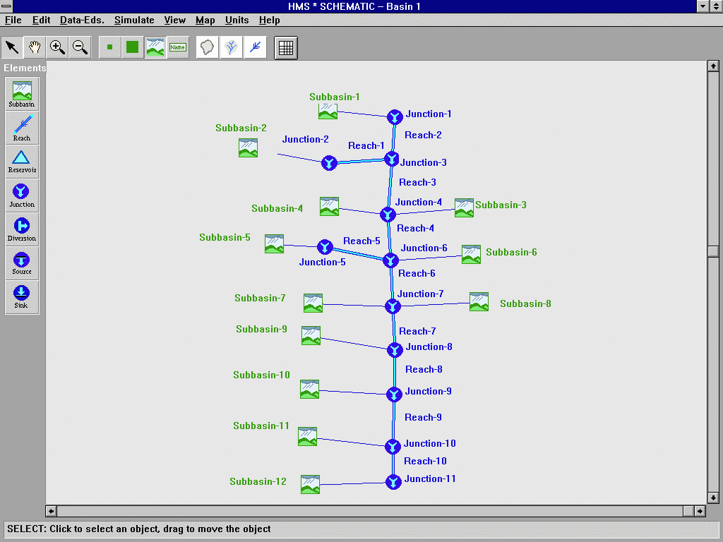
I began my study with the hopes of using the new Army Corp. of Engineers program, HEC-HMS (HMS). This program is essentially a modern version of HEC 1, a program developed by the Corp. of Engineers in 1981. HMS has a Windows interface and some features that make it more "user friendly" than HEC1. It also has the capability of creating graphical output that HEC1 lacked.
An example of this is shown above. With HMS you can visually set up the components of your watershed (icons) and enter the data for each component right on this graphical representation of the watershed.
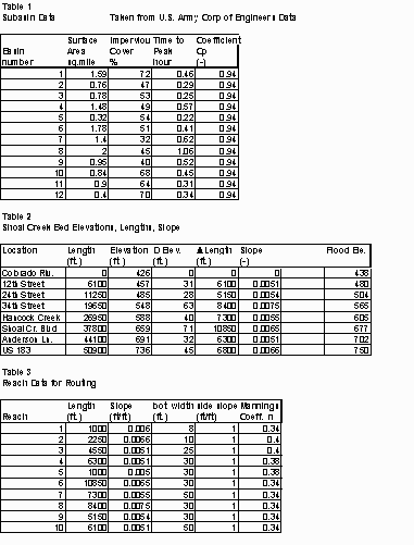
The data for the HMS model is summarized in the tables below. The physical data for the watershed is from the Corp. Of Engineers study. The entire Shoal Creek watershed had been divided into thirty subbasins with the data listed below for each subbasin. I simplified the model by combining the appropriate subbasins into one as shown in the schematic above.
A survey of the creek bottom used for flood plane analysis in the study was my source of slope and length data for the creek channels. The data for the channel dimensions (trapezoid) was gathered by measuring the creek bottom with a measuring tape at representative points on the creek and estimating the slope of the sides.
For the Basin Model I was going to use the Snyder Unit Hydrograph and the Muskingum method for channel routing. The data for these methods were available from the Corp. Of Engineers study. The data available is:
Shoal Creek Data Summary
The Mannings Coefficient (n) values I was going to use were to be in the range 0.35 to 0.4, with the 0.4 value used in the channels with more overgrowth present. These values were suggested by Dean Thomas as good estimates for the type of channel I was working with.
My work with the HMS model got as far as setting up the basin schematic with the above data for the subbasins and channels. I also determined the data for the precipitation model (which I used later with HEC1). I was unable to get the model to run after getting a lot of help for the LRC staff, presumably because of "bugs" in the beta version of the program.
I did succeed in becoming familiar with HMS format for data input and the various options for modeling. I look forward to being able to apply what I learned with the future versions of HMS and GIS data.
Some time was spent on creating my base map for the HMS model using GIS data from the CD rom of the Austin area developed by Francisco Olivera. I was going to take this data and use HECPREPRO to get it into the HMS format and import the base map into HMS. With the help of Christine Dartiguenave and Ferdinand Hellweger I got as far as isolating the data for Shoal Creek from the Austin CD and translating it the format appropriate for ArcView. It appears that the data was not suitable to be used in HECPREPRO because of data being 90 meter DEM. When this data is translated into 30 meter DEM it should be appropriate use in HECPREPRO.
Base Map From GIS
My Term Project evolved into:
It was decided that the headwaters of the Shoal Creek watershed would be the subbasin used in the model. The subbasin was defined as the part of the watershed that contributed to the outflow at Northwest Park where there is a flow gauging station.
The SCS unit hydrograph was determined to be the most appropriate mathematical relationship to use for the basin model. The SCS unit hydrograph requires the following parameters:
The Lag Time is the stuff from the book and is equal to 0.6 times the time of concentration. The time of concentration is defined as the amount of time for the whole watershed to contribute to the outflow or the amount of time for the water to reach the outlet from the furthest point from the outlet. Runoff is assumed to reach a peak at the time of concentration. The method of calculating the time of concentration for my model is the SCS lag equation:

CN= SCS runoff Curve Number
S=average watershed slope (%)
L=hydraulic length (ft), (the longest flow path in the watershed)
The time of concentration calculations were done on a spreadsheet using various curve numbers, lengths and slopes. This calculation is only for illustrative purposes. From investigation of the subbasin, the use of this equation would not be adequate to accurately represent this subbasin. Much of the flow through the outlet at Northwest Park is routed through channels which is not accounted for with this equation. Below is an example of the spread sheet calculations for time of concentration:
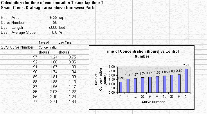
The curve number is the parameter used by the model to estimate the potential maximum retention of rainfall. In other words, with the Curve Number the model determines the amount of excess rainfall that will result in direct runoff. The Curve Number depends on soil type, land use and antecedent moisture conditions. For the Shoal Creek watershed the soil type is either Group C or Group D throughout the watershed. The land use is urban with a mix of industrial and dense residential development. A value in the range of 92-95 is a reasonable estimate for the Curve Number.
The slope used was an average of the creek bottom slopes calculated from length/elevation data taken from the Corp. Of Engineers study. The length value to use in this equation was difficult to determine. The furthest point from the outlet for this basin is approximately 19,000 feet. This value of length would not be representative of the length intended for this equation since, judging from the topographic maps and seeing the basin, most of the flow through Northwest Park has traveled a considerable distance in channels. Therefore I consider a length of approximately 9500 feet to be more representative of the basin.
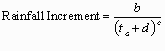
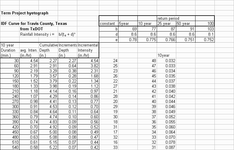
Design storms are precipitation patterns used for hydrologic modeling. Design storms are based on historical precipitation data for the area of interest. The design storm used for the input for the model is the alternating block hyetograph. The incremental depth is calculated using discrete time intervals. These values were determined by the TxDOT IDF curve equation for Travis County.
Using a spreadsheet the incremental rainfall depth is calculated and sorted. A design storm of any frequency or duration can be calculated and converted to an alternating block hyetograph. See the sample spreadsheet below.
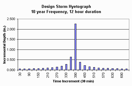
The hyetograph can be shown graphically as follows:
Upon determining the parameters above the data was set up in the format necessary for HEC1. The illustration below is a typical HEC1 input file used in my study.
With the basic HEC1 model set up I then experimented with the model by methodically changing various parameters in the model and observing the changes in the output. The following parameters were explored:
The output from HEC 1 is in the form of a simple text file with the output data in tables. The tables were inserted into Excel where they were rearranged into a useful form for analysis.
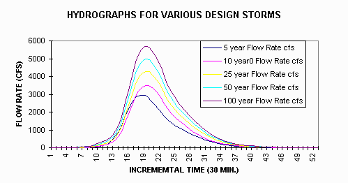
Keeping the Curve Number and the time of concentration constant, 5 different design storms were run in the model. The following graph illustrates the different resulting outflows for each design storm. The 100 year storm had the highest peak and volume (the area under the curve) and the 5 year storm had the lowest. They each had the same duration time.
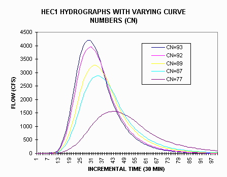
A range of curve numbers were run in HEC1 using a 5 year design storm of 12 hour duration. The following hydrographs resulted. The higher curve numbers result in a larger amount of runoff and therefore a higher peak flow and flow volume. The curve number of 93 would be representative of the Shoal Creek watershed because of it being an urban watershed with substantial development. The curve number of 77 would be representative of a undeveloped watershed with good soil infiltration and slower overland flow velocity. Note how the peak of CN77 is much lower and the curve is flattened out.
Keeping in mind that lag time is equal to 0.6 times time of concentration, note the effects of variations in the lag time on the outflow hydrograph. A smaller lag time (smaller time of concentration) results in a higher peak flow over a smaller time interval. The peak flow occurs very close the time of peak rainfall (where the curve is almost vertical). As the time of concentration is decreased the peak flow and the peak rainfall intensity get closer together.

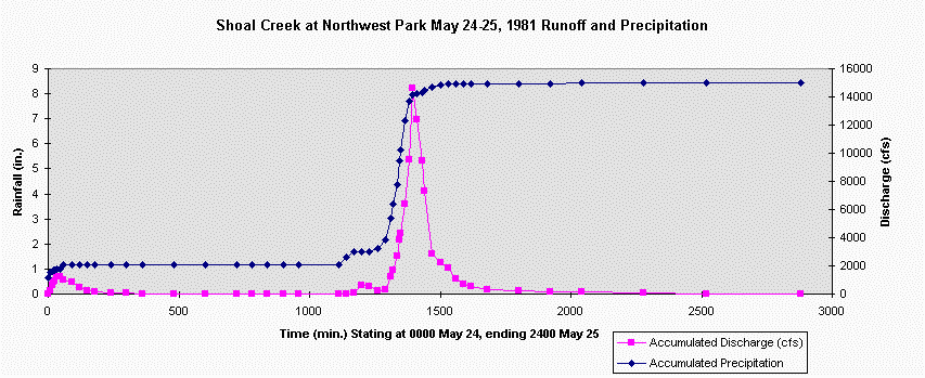
Using the data from the USGS study I created the hydrograph for Northwest Park, May 21, 1984. The graph below shows the outflow hydrograph and the accumulated rain total for the period. Note the rainfall that occurred the day before the flood event. It was enough rain to saturate the soil and cause a higher proportion of the rainfall that occurred the next day to runoff. In terms of the HEC1 model this situation would cause the Curve Number to be higher due to antecedent rain. One consequence of a higher curve number is that the time of concentration is lower as can be seen in the equation for time of concentration above.
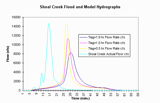
The graph below is the results of my first calculations of the time of concentration for the model using two different values for the CN. The two model hydrographs are plotted with the actual Shoal Creek hydrograph. The design storms are 100 year storms, which ,according to the data, represents the Memorial Day storm.
The reason the peak flow for the model is lower than the actual peak flow is the time of concentration was too high. I believe that this is because the equation I was using was not appropriate for this particular watershed. The parameter I believe that most effected the outcome was L, the hydraulic length of the watershed. A more accurate time of concentration can be found by calibrating the model with more actual rainfall events.

The graph below shows the model output with a variety of values for the time of concentration. As the time of concentration was decreased the model represented the actual event more accurately. It would be interesting to see how the model compared to other storm events with this value for time of concentration.
Go back to Charlie Kaough's web page
Go back to Dr. D.R. Maidment's web page