Summary

Table of Contents :

• Overview
• Project procedures
• Building the stream network
• Processing the DEM
• Defining control points
• Developing the hydrologic parameters
• Output
• Conclusions
• Future Work

Overview.

    Naturalized flows at gaged control points are then distributed to other ungaged control points in the model.  In past projects of this kind, flow distribution has usually been based on a drainage area ratio between the known and unknown points.  For the WAM project, additional watershed parameters are used to accomplish flow distribution.  The mean annual precipitation and curve number in each drainage area are calculated and used as parameters in a modification of the NRCS curve number equation.    To model all 23 river basins in Texas, thousands of control points will be established.  Geographic Information Systems (GIS) can be used to develop geospatial databases for these river basins and automate the task of determining the watershed parameters : drainage area, mean annual precipitation, and curve number.  The Center for Research in Water Resources (CRWR) at the University of Texas at Austin has developed procedures using the ArcInfo and ArcView software packages to do this work.

    The basic data set necessary to perform this work is a Digital Elevation Model (DEM).  A DEM is an equally-sized cell mesh of elevation values over an area.  The eight point pour model is applied to the DEM to determine flow direction and drainage areas across the terrain.  The eight point pour model simply assumes that water will flow from cell to cell in the direction of steepest descent.  The accuracy of DEMs becomes more suspect in flatter areas, coastal areas for instance.  There are inherent uncertainties in the elevation data.  In flat areas, difficulty in applying the eight point pour model and uncertainties in the elevation data can lead the DEM to produce very different stream and drainage representations than what ground truth (e.g. maps or aerial photography) shows.  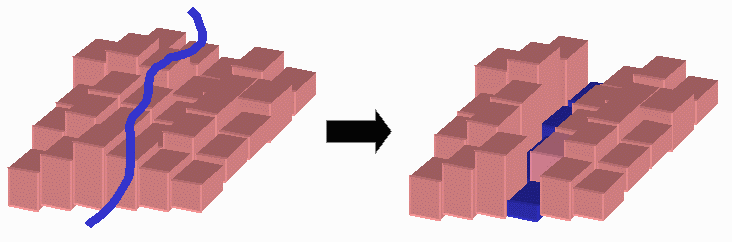At CRWR, a method has been developed to effectively "calibrate" the application of the eight point pour model to a DEM to an observed channel system.  In this process, "burning" the DEM, a vector representation of the channel system is overlaid on the gridded DEM.  DEM cells that intersect the channel vectors are effectively lowered by a large amount, in effect digging a trench in the DEM for the observed channel system.

    CRWR is also working on a TMDL modeling project for the state with similar needs.  Out of these projects, a concept has evolved of developing and working with stream networks in the basins.  Stream networks represent the channel system in a basin as a series of reaches, such that each reach is connected to only one downstream reach.  In developing the stream network, mapped networks, in this case the EPA River Reach Files Version 3 (RF3), are edited to remove unecessary features and add additional reaches as necessary.  USGS Digital Raster Graphics (DRGs) provide a reference for editing the stream network.  DRGs are scanned USGS topographic maps.  The GIS stream network coverage is overlaid on the DRG to identify additional channels and resolve editing questions.

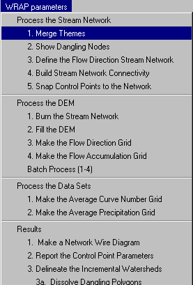
    An ArcView menu has been prepared to assist in this work.  It performs most of the functions necessary to read the hydrologic parameters of interest from input grids.  In some cases, I was not able to code a function into an ArcView Avenue script, and, at this time, ArcInfo is still necessary for a few steps.  It may be possible to perform all of the steps in ArcView, but it will require more Avenue expertise than I have to make this happen.

Back to Table of Contents

Project Procedures.

    1. Building the stream network

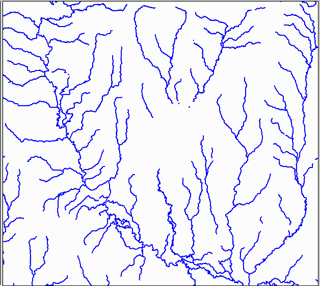
The stream network is based on the EPA RF3.  These can be downloaded (by HUC) from the EPA BASINS web site at http://www.epa.gov/OST/BASINS, under "Downloads."  The raw RF3 file looks like this :


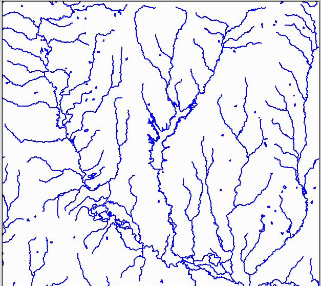
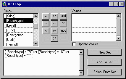
The RF3 file contains a lot of detail : shorelines of open water bodies, braided streams, and small water bodies.  Unfortunately, this detail makes it unusable for burning the DEM.  So the detail is removed by querying the RF3 attribute field, "Reachtype."  This field has a letter code describing each segment in the file.  As a first step towards making a stream network, the segments are queried for those that are true river reaches, "R", start reaches, "S", or terminal reaches, "T".  In ArcView, the Theme/Query tool  is used.

The result looks like this :

For open water bodies, the USGS has identified the centerlines and produced a GIS coverage of them.  This coverage is merged with the result of the query above. The menu function, "Merge Themes," will do this.  The Avenue script is "wrap.mergethemes".

When merged, the endpoints of the centerlines will not exactly match the endpoints of the exisiting RF3 segments.  There are several options to solve this problem.  The first is to manually fill all of the disconnects with the snap procedures described below.  The second is to not actually merge the coverages, rather to use the centerlines as a guide and manually enter the entire centerlines, again, snapping the endpoints as you go.  Finally, you may try to resolve the gaps using automated snapping functions in ArcInfo (such as the command, "matchnodes") or by using a clean and build of the topology that will be described below.

Now, manual editing must be done to reduce braided networks, parallel reaches, and cross channels to produce the network model of a single downstream reach.  Manual editing is done in ArcView using the snap features.  A detailed description of theme editing and snapping in Arcview is available through the ArcView help menu.  To use snapping in ArcView you must begin editing the theme, with Theme/Start Editing.  Then under Theme/Properties/Editing you click on both the general and interactive snapping checkboxes.  This brings up the snapping tool on the tool bar.  The snapping tool enables you to use the cursor to define the current snapping tolerance.  Interactive snapping enables lines to be specifically snapped to features such as vertices and endpoints.  The selections are made from a pop-up menu initiated with the right mouse button.

Manual editing involves some judgement by the user in selecting where to define a channel (e.g. through a braided stream network).   The DRG is used to provide some reference.  A DRG is a scanned copy of the USGS quad topographic map :


There is a problem in adding lines to the existing coverage.  As they are added, the snapped nodes are identified in the topolgy as dangling nodes.  Apparently, even though the nodes are snapped to an existing feature, they are input with a different elevation than the original nodes, and are therefore dangling.  This is a feature inherent in ArcInfo/View topology that was intended to allow for description of things such as highway over and underpasses.  To produce a clean stream network, however, it is desirable to remove these internal dangling nodes.  This can be done by building the coverage in ArcInfo as a polygon coverage.  Arcs built into polygons have all nodes collapsed to the same elevation.

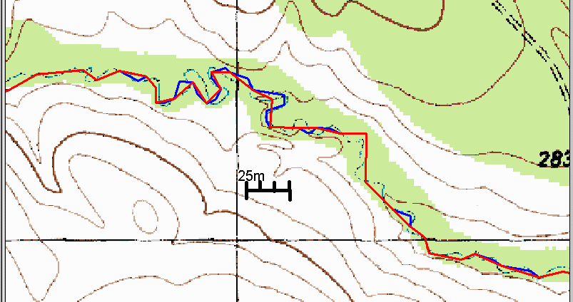
Before running build, however, you will have to clean the coverage.  This has two effects.  It will close small gaps in the network and it will make minor modifications to the network as it removes some vertices from the lines.  The effect of closing gaps is very desirable as it can save much time from doing so manually.  Modifications to the stream network are not desirable but the effect appears to be relatively minor and basically straightens the channel.  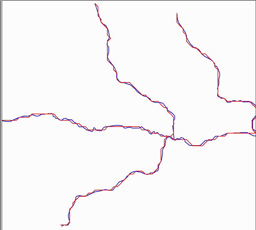The purpose of the stream network is to condition the DEM, and the resolution of DEMs along with the nature of the eight point pour model have the effect of producing straightened channels in the DEM stream definition anyways.  The screen below shows the original stream network in blue, with the cleaned network superimposed in red.  The scale shows that most modifications are on the order of 25 meters maximum difference.



When all edits have been completed the network should be checked for gaps, errors, and undesired segments.  This may be done using the menu function "Show Dangling Nodes", or with the "Ol' Bex" tool.  The avenue script is "wrap.dangles".

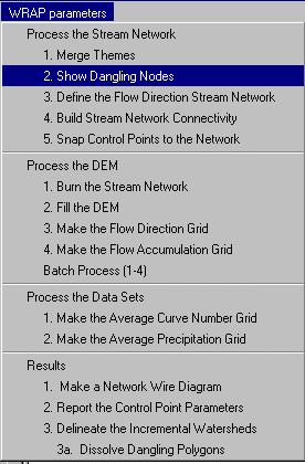
The function identifies the dangling nodes in a line theme.  The coverage is examined quad by quad and any remaining errors fixed.  The only remaining dangling nodes should be the from nodes of start reaches.

At CRWR, more stream network processing functions have been developed, but they not currently necessary for this project.  You can learn more about them in Kim Davis' term project report at http://www.ce.utexas.edu/stu/daviskm/outline.htm.

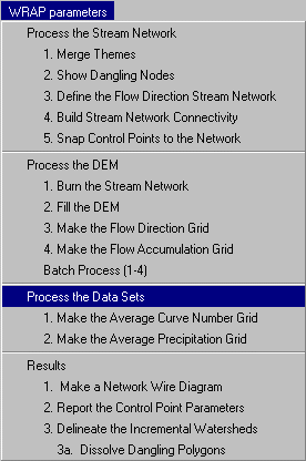
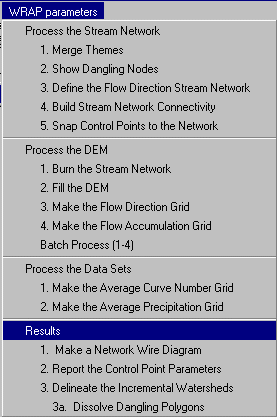
DEM processing for this project is basically the normal procedure of filling sinks in the DEM, and creating the flow direction and flow accumulation grids.  Two things are done differently in this project.  First, the stream network is burned into the DEM. Second, a coverage showing the flow direction path of the stream network is produced.  The DEM processing functions are included in the menu section, "Process the DEM."

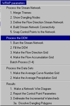
The stream network is burned with the script, "wrap.burn."  This procedure is described in an exercise developed by Dr. Francisco Olivera at http://civil.ce.utexas.edu/prof/olivera/peru/peru.htm. All cells in the DEM are raised by a large constant, except for those underlying the stream network, which keep their original elevations.  This process effectively digs a trench in the DEM following the stream network.


The burned DEM then becomes the basic grid to fill, and run flow direction and flow accumulation. The scripts used are : "wrap.fill", "wrap.fdr", and "wrap.fac".  A DEM batch processing function will also be included, but is still under construction.

Once the DEM has been processed, the DEM stream network can be defined.  In the past, DEM streams have been defined by applying a threshold value to the flow accumulation grid.  A different approach is taken in this project.  If the vector stream network is free of gaps and has had its topology built to correct interior dangling nodes, the remaining dangling nodes will be the start points, or headwaters, of the network.  These nodes may be used to define the DEM stream network from the flow direction grid.  The result is output as a line them rather than a grid.  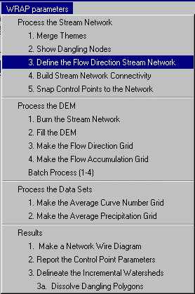The menu function is "Define the Flow Direction Stream Network". The Avenue script is "wrap.fdrstreams".

The script starts at each node and returns the least cost path from the flow direction grid and the DEM for each.  The least cost path is just the same as following the flow direction grid to the basin outlet.  Since lines are returned from every node, the coverage has many overlapping lines, and can become a huge file.  This can be corrected by taking the resulting shapefile, converting it to a coverage in ArcInfo, and building it as a polygon coverage.  Building the polygon features will eliminate overlapping lines and retain only the unique arc segments.  The arc features of the coverage can then be converted into a line theme. The figure below shows the flow direction lines, in red, superimposed on the blue stream network.


 Connectivity can be established among the arcs in this network using the menu function, "Build Stream Network Connectivity". The Avenue script is "wrap.strmsort".

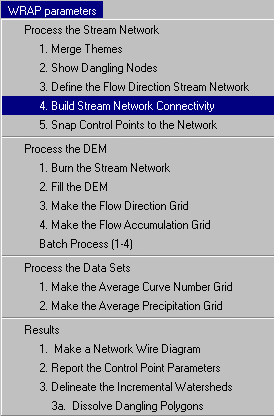
 This function assigns an arc ID to each arc in the network, and then, for each arc, determines the next downstream arc.  The arc ID and next downstream arc ID are written to the theme's attribute table.

The contractor who will actually model the basin supplies a listing of control points to be used.  Most of the control points are locations of water rights diversions and USGS stream gages.  Water rights diversion locations are provided in a shapefile from TNRCC.  USGS gage locations are available from latitude and longitude coordinates available from the USGS web site.  Additional control points can represent water quality segments, return flow locations, and other points of interest.  Locating these control points is a challenge.  The DRGs provide a good reference for communicating with the contractor.  Using them enables us to send hardcopies of the maps electronically and mark locations on the map, so there is no uncertainty in location, versus just sending a latitude and longitude for example. Control points are entered using the control point tool, .

The control points also must be located correctly on the flow direction path to produce accurate parameters.  The flow direction stream coverage can be used as a guide.  To insure that control points are located on the flow direction path, a snapping function has been included, "Snap Control Points to the Network".  The Avenue script is "wrap.snappnts".

This function operates on the entire control point coverage.  In some cases, especially at stream junctions, control points may be snapped to a position that produces results differently than desired.  For example, a control point may be placed just upstream of a junction to capture the drainage area of a tributary, but the snapping function may then snap it to the junction vertex, capturing the drainage area of the main stem and the tributary.  To help in identifying and correcting these errors, two aids are planned.  First all control points that are snapped to a junction node will be copied to a separate theme so they can be checked for accuracy.  Second, a tool will be available ( ) to snap individual points, so the snapped coverage can be edited.  These functions are still under construction.

In a few cases, the stream network cannot be adequately represented by the DEM.  In these cases some combination of control points may have to be used to capture the desired drainage area.

 The drainage area to a control point is simply defined from the flow accumulation value at that point multiplied by the cell size.


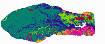
The curve number grid for the project is taken from the Blacklands Research Center in Temple, TX.  This grid was produced by combining the USDA/NRCS STATSGO soil coverage with the USGS LULC coverage.  A lookup table was used to translate the combinations of soil and land use into curve numbers using the 1972 SCS Engineering Hydrology Handbook as a reference.  The LULC and STATSGO files are both 1:250,000 scale map products, so the resulting curve number grid is relatively coarse compared to the DEM and stream network.  A few very small watersheds defined in the project so far have produced low curve numbers (e.g. 25 and 40), leading to some doubts about the precision of this data.  However, this is the best geospatial data presently available for calculating curve numbers.  The curve number grid is resampled to the same cell size as the DEM and further processed to determine average curve numbers.

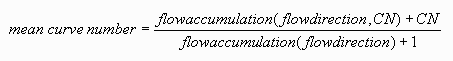
The mean curve number of several incremental watersheds may be calculated by summing the incremental weighted areas and dividing the result by the total area.

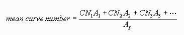
 This calculation may be reproduced in GIS using a weighted flow accumulation function.  A weighted flow accumulation request returns the sum of the values in all of the cells on the value grid within the flow accumulation area of the current cell.  When divided by the regular flow accumulation function this returns the average curve number of the watershed above the cell.  This method is identical to the averaging of incremental watersheds above, where the incremental areas are each equal to one grid cell, and the total area is the total number of grid cells in the watershed.  By adding the terms CN in the numerator and 1 in the denominator, the function just returns the CN of the current cell if it has a flow accumulation of zero.

By running this function on the curve number grid, a new grid is produced where the value of each cell is the average curve number of the watershed draining to that cell.

A grid of annual average precipitation is taken from the Oregon State University PRISM project.  This grid is processed in the same manner as the curve number grid, producing an areal weighted mean precipitation grid.

 The menu section, "Process the Data Sets" calculates the weighted curve number and precipitation grids from the base curve number and precipitation grids.

    5. Output

Output results are prepared with the menu section "Results".

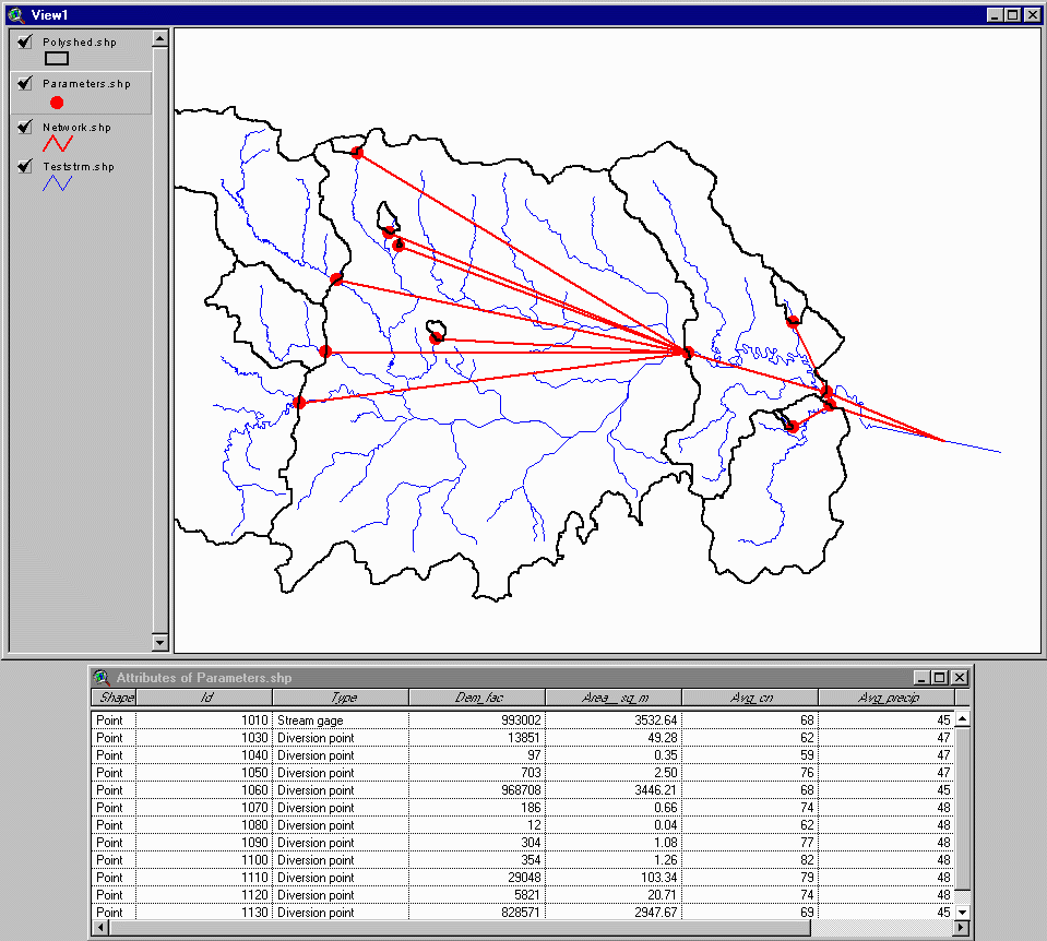
"Make a Network Wire Diagram" connects each control point to the next downstream control point (or outlet) with a straight line.  The Avenue script is "wrap.network".  This can be a useful tool in visualizing a network with hundreds of control points.

The parameters from the flow accumulation and weighted curve number and precipitation grids at the location of each control point are read and written to a new coverage.  This coverage is called parameters.shp and is just a copy of the control point coverage with fields added for area, mean curve number, and mean precipitation. The menu function, "Report the Control Point Parameters", does this.  The Avenue script is "wrap.parameters".

Finally, the function "Delineate the Incremental Watersheds" produces a polgon theme of the incremental watershed for each control point.  The Avenue script is "wrap.watershed".  The watershed theme is necessary to conduct quality control of the drainage areas.  The watershed theme can be projected to the appropriate UTM projection and the watershed boundaries overlaid on DRGs to make sure the drainage areas have been correctly defined.  A useful rule of thumb seems to be 1000 DEM cells.  Watersheds below this size are very sensitive to the correct definition of the stream network.  In these cases, all of the upstream and neighboring tributaries that can be identified from the DRG should be added to the original vector stream network prior to burning the DEM.
One sub-item, "Dissolve Dangling Polygons," is needed here to eliminate small diagonal polygons that are erroneously produced in the watershed definition.  The Avenue script is "wrap.dissolve".
 

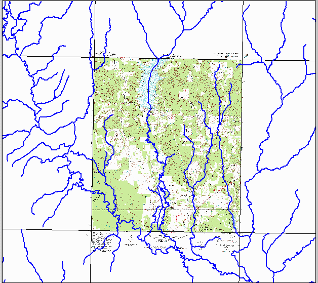
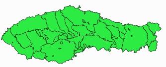
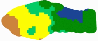
Results for a small test basin are shown here :

 

Conclusions.

Back to Table of Contents

Future Work

Back to Table of Contents

Go to CE394K2 term papers

Go to my home page