
CE 394K.3 - GIS in Water Resources
The original focus of this project was to conduct a hydrologic analysis for a TxDOT (Texas Department of Transportation) highway drainage structure in the Wichita Falls TxDOT District in Texas as part of a project I am working on at the Center for Research in Water Resources (CRWR). However, specific details of the TxDOT project were not known during the time frame of this GIS class project. Instead I will carry-out a similar analysis for Wichita County, located in the northern part of the TxDOT district. In this analysis, I hope to gain skills required to conduct a similar hydrologic analysis for TxDOT when the scope of the project is defined.
In the first stage of this project I use ArcView and its Spatial Analyst extension, along with a spatial data preprocessor, CRWR-PrePro, developed by CRWR, to calculate hydrologic parameters of the floodplain. With a digital elevation model input (DEM) and a digitized stream network, it is possible to delineate a drainage system using this software. The watersheds and stream networks created from the DEM are also the primary inputs to the HEC-HMS surface hydrologic model. HEC-HMS (Hydrologic Modeling System) is a flood package used to calculate precipitation runoff developed by the US Army Corps of Engineers Hydrologic Engineering Center .
The most essential data required for this analysis are a digital elevation model (DEM) and a digitized stream network. These data can be obtained once the HUC (hydrologic unit code) is known. All data were obtained free-of-charge over the internet, or from the CRWR database (these data can alternatively be downloaded over the internet).
The location of TxDOT Wichita Falls district, and information regarding this district, can be found on the TxDOT web site http://www.dot.state.tx.us/insdtdot/geodist/wfs/wfsdist.htm. This northern Texas area is formed by seven counties: Archer, Baylor, Clay, Cooke, Montague, Throckmorton, Wichita, Wilbarger and Young as shown in Figure 1: Wichita Falls TxDOT District.
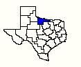
Figure 1: Wichita Falls TxDOT District (highlighted in blue)
The HUC representing Wichita county is 11130206. This is an arbitrary area of analysis for the reason mentioned above (minimal information on the actual TxDOT project is currently known). Details on hydrologic cataloging units can be found on the USGS webpage: http://water.usgs.gov/GIS/huc.html. Additional information regarding this particular cataloging unit can also be found on the EPA website. HUC 11130206 covers an area of 1012.07 square miles. Figure 2: HUC 11130206 shows this cataloging unit in relation to Texas and the city of Wichita Falls.
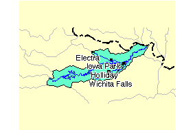
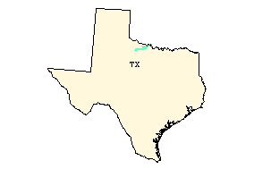
Figure 2: HUC 11130206
All the data were projected into TSMS (Texas Standard Mapping System) Albers coordinates. The parameters of TSMS Albers are shown below:
Data preparation involved using ArcView and its Spatial Analyst extension, CRWR-Raster extension, ArcInfo and CRWR-PrePro. ArcInfo was used to project the grids, and the ArcView Projector! extension to project the shapefiles.
The first data modification made was buffering the cataloging unit using the ArcView Theme/Create Buffers command. This buffer of 5000 meters will account for water flowing into HUC 11130206. The next step involved obtaining the digital elevation data (or digital elevation models, DEMs) for cataloging unit 11130206. The resulting 30-m DEMs are 9934, 9835 and 10034 where the first 2-3 digits represent west longitude, and the last two digits north latitude in geographic coordinates. These DEMs correspond to the USGS 1:24,000 scale topographic quadrangle map series. I obtained these three DEMs from the CRWR database, but these can also be found on the National Elevation Dataset webpage http://edcnts12.cr.usgs.gov/ned. The grids were then merged using ArcView, and then projected in the the TSMS Albers coordinates using ArcInfo. Figure 3: DEM and Buffered HUC 11130206 shows the merged DEMS in relation to the buffered cataloging unit.
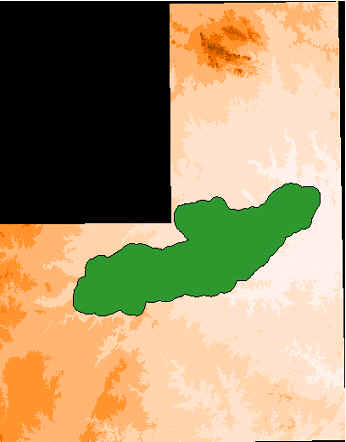
Figure 3: DEM and Buffered HUC 11130206
Next, I downloaded the corresponding National Hydrography Dataset (NHD) digitized stream network from the NHD website http://nhd.usgs.gov. The following picture shows the NHD stream network, HUC 11130206 and buffered HUC 11130206. The waterbody used in this project was route.rch. As the network was comprised of many unnecessary segments, this was edited in ArcView. Figure 4: Stream Network portrays this stream network and buffered cataloging unit.
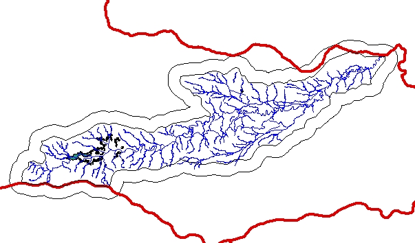
Figure 4: Stream Network
After the HUC was buffered, the route.rch shapefile was extended so that the water would be able to flow out of this unit as shown in Figure 5: Extended Reach below.
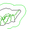
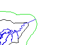
Figure 5: Extended Reach
The next stage was to collect stream gage information. This can be downloaded free of charge from the USGS web site www.usgs.gov. Figure 6: Animated Gage Hydrographs shows the station numbers and the date for both stations.
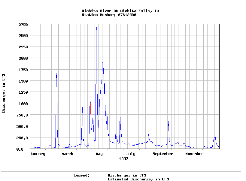
Figure 6: Animated Gage Hydrographs
To create a shapefile with these data, I defined a table containing an ID, and the longitude/latitude coordinates of the gages. These numbers were converted into geographic degrees, minutes and seconds in an ArcView table. To generate a point shapefile showing the gage locations, I used the scripts icon and loaded textfile defgages.ave provided by Exercise 2: Building a Watershed Base Map. In the attributes table, I added the names and max flows (during the same day) for these two gaging stations as shown in Figure 7: Gaging Station Attributes. Station number 07312500 has a drainage area of 3140 miles2, and 07312130 which has a drainage area of 2246 miles2.
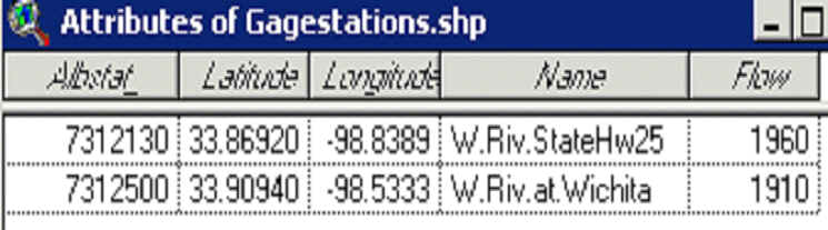
Figure 7: Gaging Station Attributes
The last step involved clipping the grid to the extent of the buffered HUC polygon using the CRWR-Raster extension and Clip by Polygon function, and this enabled me to clip the polygon to the DEM as shown below. Figure 8: Clipped DEM shows the new digital elevation model to be worked with.
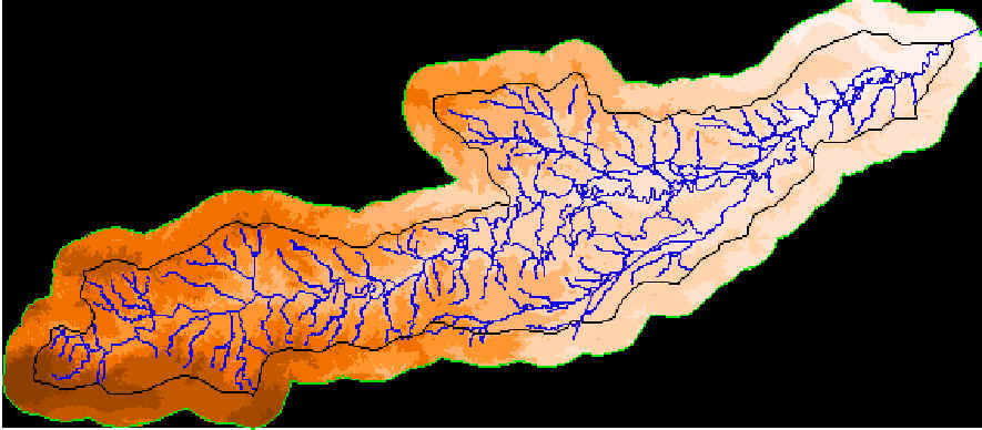
Figure 8: Clipped DEM
Now all the data are prepared to be processed.
As mentioned earlier, ArcView GIS, the Spatial Analyst extension and CRWR-PrePro are used to delineate the watersheds. CRWR-PrePro, along with ArcView and its Spatial Analyst extension can process a DEM model and delineate its streams and watersheds. A project file which contains the necessary scripts, menus and buttons for running CRWR-PrePro, prepro03a.apr, can be downloaded from the CRWR-PrePro website http://www.ce.utexas.edu/prof/olivera/prepro/prepro.htm. Once the prepro03a.apr project is opened in ArcView, input data for the HEC-HMS model can be generated by conducting a raster-based terrain analysis and raster-based subwatershed and reach network delineation. These steps followed by vectorization of subwatersheds and reach segments, and computation of hydrologic parameters allow for extraction of HEC-HMS basin file.
After setting the ArcView Anaysis Extent to the same as the clipped DEM, I used the following CRWR-PrePro commands to process: CRWR-PrePro/ Burn Streams to burn in the streams (1000 meter arbitrary elevation rise), CRWR-PrePro/ Fill Sinks to fill the sinks of the DEM, CRWR-PrePro/ Flow Direction to compute the flow direction grid, and finally CRWR-PrePro/ Flow Accumulation to compute the flow accumulation grid. These steps are all very time consuming. It is important to set the analysis extent each time the project is opened, or else the grids may not be locally consistent with one another.
Burning in the streams raises the land surface cells so that the streams delineated from the DEM match the digitized stream network (route.rch). Filling in the sinks accounts for errors in the DEM, such as pits or aberrations, that are very small. If the pits are not filled, this can result in erroneous flow directions. The flow direction function uses the Eight Direction Pour-Point model to determine the flow from each cell into its neighboring cells according to the path of steepest decent. The last computation, flow accumulation, represents the cells contributing flow to the pour-point.
STREAM DELINEATION
The next step is to identify the flow elements of the hydrologic system. After analyzing thresholds of 1000, 5000 and 10,000 I decided to choose a threshold of 5000. Once this minimum stream drainage area was determined, the segment streams were converted into stream links using the CRWR-PrePro/Stream Segmentations (Links) command. This function gives each segment a unique ID. Following this the outlets were defined with the CRWR-PrePro/Outlets from Links command. The outlet cell is the cell in each link which has the largest flow accumulation. The last part of this step was to add the gaging stations defined above. This can be done manually with the add outlets (O) tool, followed by CRWR-PrePro/Add Outlets function. Figure 10: Stream Links and Thresholds shows the outputs of these functions.
STREAM LINKS 10,000 Threshold 1000 Threshold
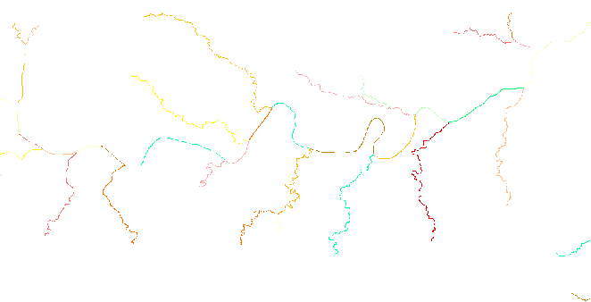
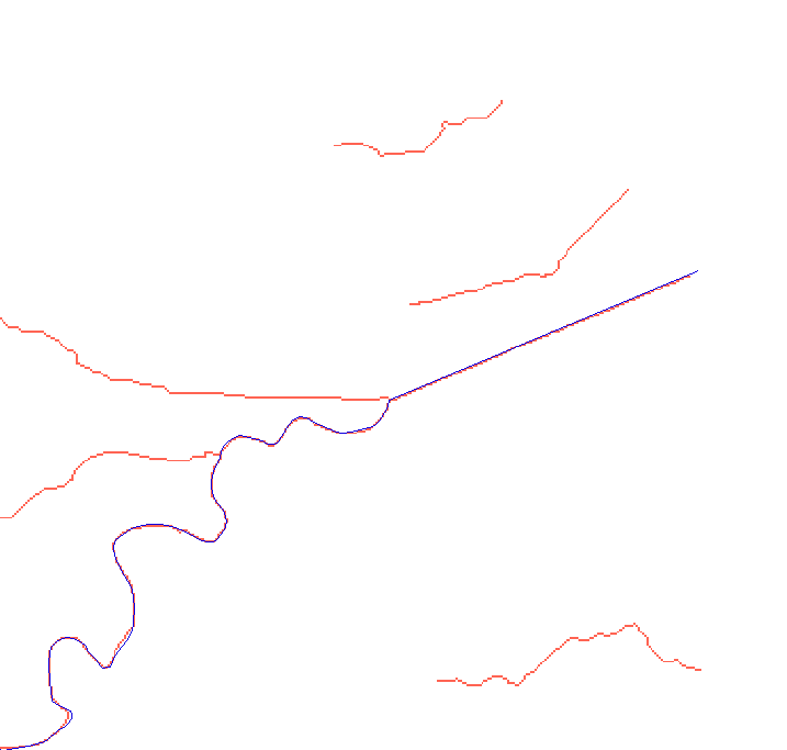
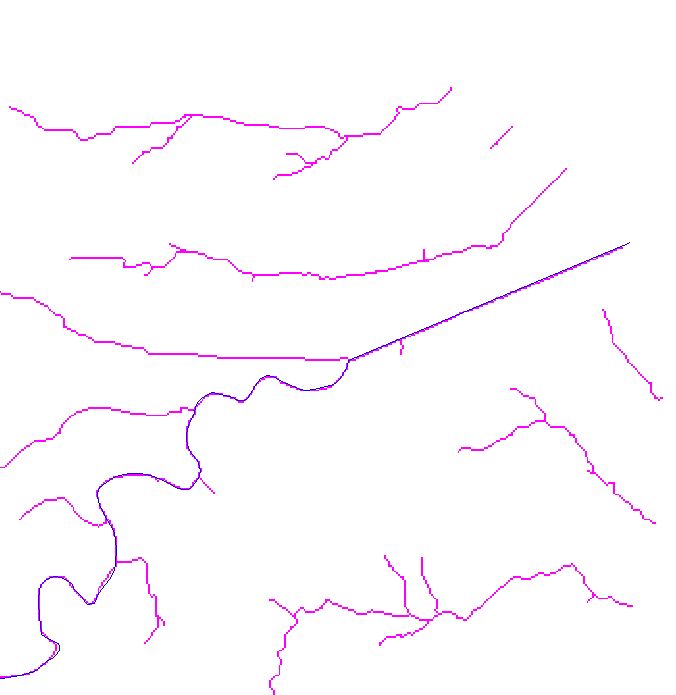
Figure 9: Stream Links and Thresholds
SUBWATERSHED DELINEATION
Identifying individual drainage areas can be accomplished using the CRWR PrePro/Sub-Watershed Delineation function. CRWR-PrePro uses all the outlets to generate one subwatershed per outlet. The next step, vectorizing the streams and watersheds using the CRWR-PrePro/ Vectorize Streams and Watersheds command, produces a shapefile of the vectorized streams and subwatersheds and transfers the grid code values to the attribute tables of the feature datasets. Figure 11: Animated Delineation Steps below shows three steps in this process: the multicolored dark-blue flow direction grid, the beige-colored subwatershed delineation grid and the teal vectorized streams and watersheds.
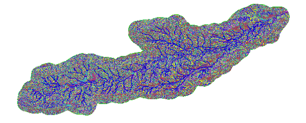
Figure 10: Animated Delineation Steps
The stream length in this step should be less than or equal to 1.41 times the cell size. Unfortunately, I found this to be the case in the vectorized stream shapefile. One option was to start all over again, and try using a higher stream threshold. As I had already started from scratch several times, I decided to instead clip an area upstream, and just focus on these manually selected sub watersheds. The main setback here is that this upstream area lacks a USGS gaging station. Figure 12: Extracted Hydrologic Subsystem represents the clipped area and new drainage system to be analyzed.
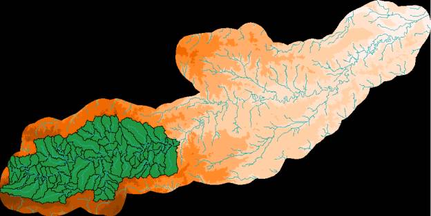
Figure 11: Extracted Hydrologic Subsystem
WRITING A BASIN FILE FOR HMS
The next step in developing a hydrologic model for this system is done by calculating the hydrologic attributes using the CRWR-Prepro/Calculate Attributes command. The abstractions method selected is SCS (Soil Conservation Service), SCS is selected for the lag-time method, and a time-step of 30 minutes is selected. The curve number grid was obtained from the CRWR database. Also needed in this process is the streamP.txt file. This was obtained from a previous assignment located on the CRWR-PrePro homepage: Developing a Hydrologic Model of the Guadalupe Basin. This table was developed for the Guadalupe basin in Texas and therefore should be changed. However, for the purpose of this project this table was not changed.
To transfer the hydrologic attributes to the schematic and basin file it is necessary to first add the following tables to the working directory: hecsub.dbf, hecjunct.dbf, hecreach.dbf, hecres.dbf, hecsink.dbf, hecsource.dbf and hecdiv.dbf. These tables can also be found in exercise Developing a Hydrologic Model of the Guadalupe Basin. Lastly, the command CRWR-Prepro/HMS Schematic is selected. The following picture shows the sink (in red) and the junctions and outlets as defined by ArcView with the newly created shapefiles. These shapefiles contain all of the relevant information for use in HMS as displayed by ArcView in Figure 13: ArcView HMS Schematic View.
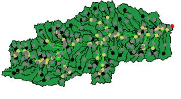
Figure 12: ArcView HMS Schematic View
HEC-HMS requires three input components: a basin component, a precipitation component and a control component. CRWR-PrePro extracts all the necessary topographic, topologic and hydrologic information and prepares an ASCII file for the basin components and precipitation components of HEC-HMS. These files create a topologically correct schematic network of subbasins and reaches attributed with hydrologic parameters, as shown in Figure 14: HMS Model. There is also a file to relate gage to sub-basin precipitation time series. However, in this case these data have not been incorporated as there are no gaging stations in this area.
Figure 13: HMS Model
Currently HEC-HMS has two different methods of incorporating precipitation data into the model. The first is user-specified gage weighing and the second is automatic determination of gage weights based on Thiessen and sub-basin polygon date sets (gridparm). Gage locations are necessary in HEC-HMS to calibrate the flows from design storms. From this stage it is possible to add precipitation data to determine a hydrograph at various points on the network.
There were several problems encountered during this project. I feel as though most of the problems were a result of inexperience in using the software. The mistakes I have made I have learned from, so that they will not be repeated! Some of these problems include the following: I didn't consistently set the Analysis Extent when opening my project on a new day (ArcView doesn't seem to save these settings), I didn't edit the route.rch file the first time I burned in the streams, I had three one-cell stream links (which could have possible been taken care of at the start by using a larger threshold), and I had too many streams for analysis using HMS (before it was clipped). Owing to these setbacks, I was not able to spend much time using HMS.
This project proved to be an excellent preparation for my thesis and introduction to the world of GIS. Future work on this project will most likely be done using the Texas Centric Mapping System/ Albers Equal Area, a current standard projection for Texas (http://tgic.state.tx.us/standards). This projection facilitates easy, accurate overlay and integration of multiple datasets. Future work will most likely involve repeating this analysis with more defined specifications and a more extensive set of data such as land use/land cover data, soils (STATSGO) data, major roads, and populated place locations.
I thank Dr. Olivera, Dr. Maidment and the CRWR second-year students for their help!
Andrysiak, Peter B. Jr. GIS Based Flood Damage Reduction Analysis Of Mill Creek, Ohio. CE394-K3 GIS in Water Resources class term project. University of Texas at Austin
Anderson, David and Olivera, Francisco. System of GIS-Based Hydrologic and Hydraulic Applications for Highway Engineering. Center for Research in Water Resources, The University of Texas at Austin. September 11th, 2000
Olivera, Francisco and Maidment, David. GIS-Based System of Hydrologic and Hydraulic Applications for Highway Engineering: Research Report 1738-6. Center for Transportation Research, Bureau of Engineering Research. The University of Texas at Austin. October 1999.
Maidment, David. Delineating the Watershed and Stream Network of the Guadalupe Basin. Developed for the s class at the University of Texas. Fall 1998.Maidment, David R. Exercise 2. Building a Watershed Base Map, CE 394K GIS in Water Resources, University of Texas at Austin, Fall 2000
Olivera, Francisco and David Maidment. Developing a Hydrologic Model of the Guadalupe Basin. Developed for the CE394-K3 GIS in Water Resources class at the University of Texas. Fall 1998.
Tanya Hoogerwerf 12/8/00