Procedure
The following is an outline of the procedure devised for extracting the drainage coverages from the DCW CD ROMs and editing them. In this procedure, data is extracted for the whole of the African continent. The Congo basin in Central Africa is subsequently used to illustrate the detailed processing required to achieve full network connectivity in the coverage.
Selecting the CDROM Tiles
The ESRI version of the DCW is composed of 4 CD ROM discs covering the areas enclosed by the following lines of longitude:
CDROM |
EXTENT (longitude) |
| DISC1 | -90o TO 0o |
| DISC2 | -180o to 90o |
| DISC3 | 0o to 90o |
| DISC4 | 90o to 180o |
Table 1: Extent of ROM Discs
The first step is to define the geographical extent of the study area, and to identify which CDROM contains the coverages of that area. The continent of Africa is enclosed by the following lines of longitude and latitude.
BOUNDARY |
GEOGRAPHIC EXTENT |
| Northern Latitude | 40o |
| Southern Latitude | -35o |
| Western Longitude | -20o |
| Eastern Longitude | 55o |
Table 2: Geographical Extent of Africa
Extracting and Merging Coverages
The CDROMs corresponding to this region are Discs 2 and 3. The data on each of
these discs is divided into tiles each covering 5o of latitude and 5o
of longitude. A separate directory is created for each tile. The directories are labeled
by a location label consisting of two letters and two numerical digits. Under each
tile directory, there are 17 vector coverages representing the layers of information
described in the table below.
Layer Name and Number |
Theme Abbreviation |
Coverage Name(s) |
| 1 Political Oceans | PO | PONET , POPOINT |
| 2 Populated Places | PP | PPPOLY , PPPOINT |
| 3 Railroads | RR | RRLINE |
| 4 Roads | RD | RDLINE |
| 5 Utilities | UT | UTLINE |
| 6 Drainage | DN | DNNET , DNPOINT |
| 7 Drainage Supplement | DS | DSPOINT |
| 8 Hypsography | HY | HYNET , HYPOINT |
| 9 Hypsography Supplement | HS | HSLINE , HSPOINT |
| 10 Land Cover | LC | LCPOLY , LCPOINT |
| 11 Ocean features | OF | OFLINE , OFPOINT |
| 12 Physiography | PH | PHLINE |
| 13 Aeronautical | AE | ASPOINT |
| 14 Cultural Landmarks | CL | CLPOLY , CLPOINT , CLINE |
| 15 Transportation Structure | TS | TSLINE , TSPOINT |
| 16 Vegetation | VG | VGPOLY |
| 17 Data Quality | DQ | DQNET |
Table 3: Digital Chart Data Layers
The Arc Info command MAPJOIN function was used for extracting and merging the drainage coverages of Africa. Click on the following links to view the respective AML programs for extracting the drainage layer data from the respective discs: AML for disc 2 and AML for disc 3. The coverages can also be merged using the Avenue script mergethm.ave. The resulting river coverage is shown in Figure 1 below.
Figure 1: Merged River Coverage for Africa
Separating Line and Polygon features
The merged coverages are initially in geographic coordinates. They must be projected on to a flat surface before any editing can begin. This is because the snap, weed and other feature editing tolerance used in Arc Info are only meaningful if the data is in flat map coordinates. This may not be significant when working with small regions but the effects can be considerable when working with large regions. The projection was done in Arc Info though the same procedure can also be executed in ArcView. The projection parameters for the Lambert Azimuthal Equal Area Projection used in Africa are listed in Table 4 below.
| INPUT |
| PROJECTION GEOGRAPHIC |
| UNITS DD |
| PARAMETERS |
| OUTPUT |
| PROJECTION LAMBERT_AZIMUTH |
| UNITS METERS |
| PARAMETERS |
| 6378137.0 |
| 20 0 0 |
| 5 0 0 |
| 0.0 |
| 0.0 |
| END |
Table 4: Lambert Azimuthal Projection File for Africa
The merged coverage was projected using the following Arc Info command:
Arc: project cover afriver1 afriverprj lm_azafr.prj
where afriver1 is the name of the merged coverage
afriverprj is the name of the projected output coverage
lm_azafr.prj is the projection file
The projected coverage is form the Congo basin is shown in figure 2 below. Notice the existence of several double lined streams lakes and straight lines marking the edges of map sheets.
Figure 2: Merged River Coverage of the the Congo Basin
The river arcs were separated from the polygons in ArcEdit, the Arc Info feature editing module. The results of this separation are shown in figure 3 below.
Figure 3: Separated River Line and Polygon Coverages of the Congo
Extracting the Centerlines of Polygon Features
After separating the river arcs from the polygons, the centerline of double lined streams and lake must now be determined and reincorporated into the river arc coverage. To do this, the polygon coverage is first edited to remove polygons that are formed by the boundaries of non-stream features such as lines of latitude and longitude and coastal shorelines. As shown in Figure 4 below, the resulting coverage contains only the polygons formed by double lined rivers, lakes and reservoirs.
Figure 4: Polygons of Double Lined Flow Channels in the Congo
The coverage of double lined channels is then converted from its original vector format to a raster grid. This step allows us to take advantage of the thinning functions available in the Arc Info grid environment. The THIN command allows us to continually chip off the cells at the outer edge of a gridded feature until the feature is reduce to a single chain (or other specified thickness) of cells . The sequence of commands for this process is as follows;
Arc: dissolve afrivpoly1 afrivpoly2 myvalue poly
The field 'myvalue' is a dummy attribute containing a value of 1 for each polygon. The dissolve command removes all the small polygons (islands) contained within larger water bodies. Convert the polygon to a grid with
Arc: polygrid afrivpoly2 afrivgrid myvalue
Cell Size (square cell): 100
Convert the Entire Coverage (Y/N)?: Y
Arc: grid
Grid: setwindow afrivgrid afrivgrid
Grid: setcell afrivgrid
Grid: afthin200 = thin ( afrivgrid , positive, nofilter, round, 4000)
Grid: afriv200 = gridline ( afthin200, positive, nothin, nofilter, round, value)
Grid: quit

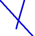
Figure 5: Raster and Vector Derivatives of Thinning
The Figure 5 above shows a section of the double lined river after conversion into raster format (in green) and the result of the thinning process in blue. The thinned raster representation can then be converted back into a single line river representation as shown in part b of the figure. From the image above, it is clear to see that centerline thus created has a lot of sharp bends which would result in a longer than expected river reach length if used in hydrologic modeling in its present state. The GENERALIZE command is consequently used to remove any unnecessary nodes.
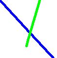
Figure 6: Effect of generalization on Vectorized Centerlines
The Figure 6 above shows the effect of generalization. The original centerline shown in blue is generalized to a more representative straight line representation. Note that the generalization is sensitive to the weed tolerance defined. For the centerlines on the water bodies in Africa, a threshold of 200 meters gave the best result. The syntax of the generalize command is as follows;
Arc: generalize afriv200 afcenterln 200 pointremove
Establishing Network Connectivity
The centerlines can now be reincorporated into the river network by simply selecting all the arcs in the stream centerline coverage and putting them into the river line coverage. The resulting coverage must then be edited manually to ensure all arcs are appropriately connected to the network. Refer to ArcView based scripts developed for the CRWR River Network Preprocessor for trouble shooting and editing tools. The Arc Edit commands listed below may also be used.
Initiate the Arc Edit environment with the command
Arc: arcedit
Arcedit: display 9999
Arcedit: edit rivercov arc
specifies the edit coverage and feature type. The edit distance, a measure of how close one has to get to a feature before being able to select it, is specified with
Arcedit: editdistance
Similarly, the snap distance is measure of how close two features must be to each other before they are automatically snapped together. The snap distance is specified for nodes and arcs respectively with
Arcedit: nodesnap closest *
Arcedit: arcsnap closest *
Some commonly encountered mistakes are listed below along with ways to correct them.
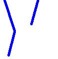
1) Undershoots occur when an arc which is supposed to intersect another arc stops short of its target. As illustrated below, the way to correct an undershoot is to select the arc and extend it using the commands listed below.
 |
 |
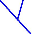 |
| Arcedit: | select | extend |
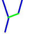
2) Overshoots arise when an arc extends past the arc it is supposed to be linked to. Overshoots can be corrected by coverting the arc to an undershoot and extending as described in (1) above.
 |
 |
 |
 |
|
|
|
| Arcedit: | select | split | select | delete | select | extend |
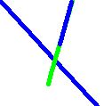
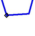
3) Missing arcs can be replaced by on screen digitizing using the ADD command.
 |
 |
| Arcedit: | add |
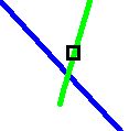
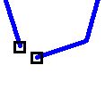
4) Mismatched nodes can be brought together by setting the edit feature to node and moving one of the nodes to coincide with the other.
 |
 |
| Arcedit: ef node | move |
To save edits (do this often to avoid losing edits),
Arcedit: save
Build the resulting line coverage to reestablish arc topology and to update the values in the arc attribute table.
Arc: build rivercov
It is important to be able to check make sure that the network is fully interconnected. This can be done by running a trace in ArcPlot as follows:
Arc: arcplot
Arcplot: display 9999
Set the map extent to that of the river coverage with
Arcplot: mapextent rivercov
To display the arcs in the river coverage, type
Arcplot: arcs rivercov
Begin the trace with
Arcplot: trace direction rivercov upstream downstream *
(select an outlet from the display by clicking on it)
To display the results of the trace, type the following sequence of commands
Arcplot: linesymbol 2
Arcplot: readselect downstream
Arcplot: readselect upstream keep
Arcplot: arcs rivercov
The arcs that are not connected to or pointing away from the outlet will be shown in white. All other arcs will be shown in red. Figure 7 below showns and example of misoriented arcs in a network.
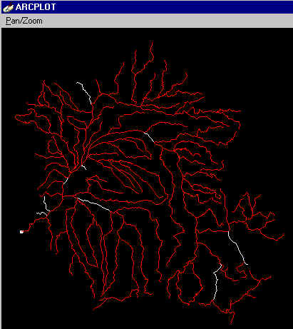
Figure 7: Congo Basin Network with Misoriented Arcs in White
To correct the orientation of misoriented arcs, open the coverage in Arc Edit as before.
Arc: arcedit
Arcedit: display 9999
Arcedit: edit rivercov arc
Select all the misaligned arcs using the select many command
Arcedit: select many
Now change the orientation of all selected arcs with
Arcedit: flip
The orientation of the arcs will now be corrected so that they point towards the outlet. Save the coverage and exit Arc Edit as before. Redo the trace to confirm that all arcs are now connected to the outlet.
The editing of the editing of the DCW stream will require a major effort involving
several individuals. However, the results of applying a similar approach to clean up the
ArcWorld dataset in the Congo Basin are shown in Figure 7 below. The resolution of the
river representation in the ArcWorld dataset is 1:3,000,000.
Figure 8: Congo River Network from Arc World
The underlying gray line is the original ArcWorld data set while the edited river network of the Congo is shown in blue.