The FAO/UNESCO Water Balance of Africa is an effort undertaken jointly by the Center for Research in Water Resources of the University of Texas at Austin, the UN Food and Agriculture Organization, and UNESCO, for the purpose of better assessment and planning of the water resources of Africa.
The project has three main components:
The Niger River basin in West Africa is used as a case study region for the database and model development. Monthly soil water surplus is calculated using the Thornthwaite soil water balance model, although the evaporation computation has been modified to include a spatial database of net radiation obtained from the Earth Radiation Balance Experiment. These water surpluses are transferred onto subwatersheds of the Niger Basin and routed through its river system using the Muskingum method. The flow from the subwatershed to the river moves partly through the subsurfacesystem and partly through the surface system, each delayed in time by a differing amount. 30'grid of mean monthly precipitation and temperature from Legate-Willmott global climatology.
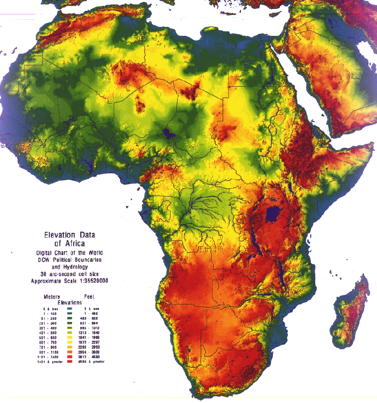
The work makes use of a gridded representation of the land surface
terrain of the continent in the form of a 30" Digital Elevation
Model of Africa, developed by the US Geological Survey in Sioux
Falls, South Dakota, with the cooperation of the UN Environment
Program.
The data region used here is centered on Morocco and extends from
approximately (14W, 26N) to (1E, 37N), including both the oceans
and the land surface.>
The main goal is to demonstrate how simple potential evaporation
and soil-water budget calculations can be made within ArcView
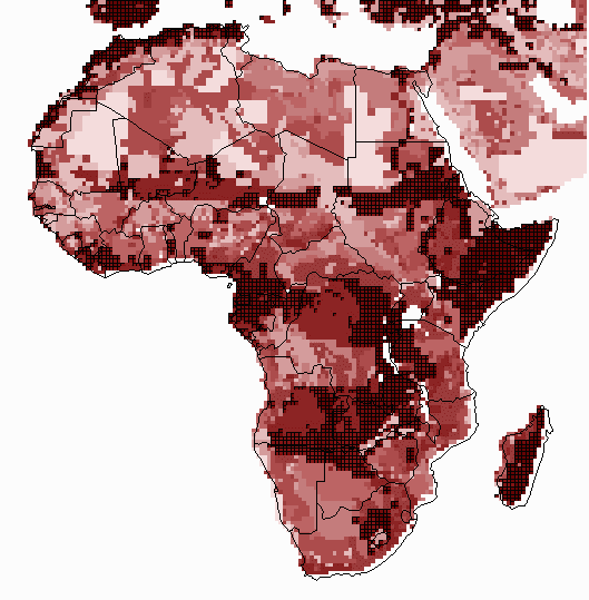
Mean monthly temperature and precipitation estimates interpolated onto a 0.5 by 0.5 mesh were obtained from Cort Willmott at the University of Delaware. These data come from the "Global Air Temperature and Precipitation Data Archive" compiled by D. Legates and C. Willmott. The monthly precipitation estimates used in this study were corrected for gage bias. Data from 24,635 terrestrial stations and 2,223 oceanic grid points were used to estimate the global precipitation field. The climatology is largely representative of the years 1920 to 1980 with more weight given to recent ("data-rich") years (Legates and Willmott, 1990).
The raw data obtained from the University of Delaware were downloaded
via ftp in formatted text files. FORTRAN and AML were used to
generate a polygon coverages (converted to a shapefile to simplify
ftp transfer) of these data, shown here below.
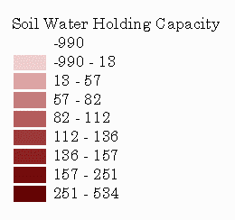
Global estimates of "plant-extractable" water capacity (water-holding capacity) on a 0.5 degree grid estimates were obtained via anonymous ftp from the USGS Geophysical Fluid Dynamics Laboratory. This data set was compiled for a Master's thesis written by Krista Dunne at the University of Delaware. Information about sand, clay, organic content, plant rooting depth, and horizon thickness was used to estimate the water-holding capacity. An important source of data used in this analysis was FAO's Digitized Soil Map of the World (FAO, UNESCO, 1974-1981). The global average soil water-holding capacity estimate is 86 mm.
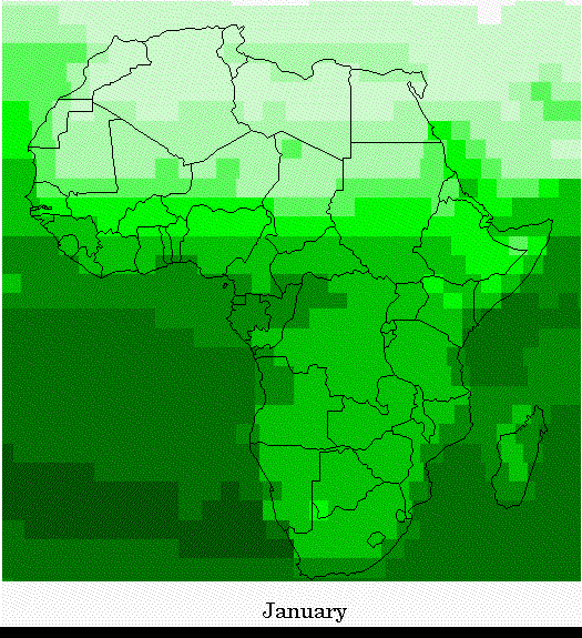
Global mean monthly net radiation data generated as part of the International Satellite Cloud Climatology Project (ISCCP) are now available for a 96 month period extending from July 1983 to June 1991. The data are given on the ISSCP equal-area grid which has a spatial resolution of 2.5 degrees at the equator. Monthly average and mean annual and mean monthly values of net radiation were computed for this 8 year period. To make computations easier, the radiation data were resampled to the same resolution as the climate and soils data (0.5 degree cells).
The formula used for computing the potential evaporation is:
Ep = 1.3 (d / (d+g)) Er
where Ep is the potential evaporation rate in mm/mo., d is the gradient of the saturated vapor pressure curve in kPa/degree C at the prevailing temperature T in degrees C, g is the psychrometric constant in kPa/degree C, and Er is the water evaporation equivalent of the net radiation in mm/day. The values of d and g as a function of temperature aregiven in Table 4.2.1 p. 4.4 of the Handbook of Hydrology, (McGraw-Hill, 1993, ed. by D.R. Maidment). The value of Er is given by:
Er = 86,400 Rn / L
where Rn is the net radiation in W/m2, L is the latent heat of vaporization of water in J/kg, and 86,400 is the number of seconds in a day. The value of L is given by:
L = 2.501 x 10^6 - 2361 T
where T is the prevailing temperature.
Another Avenue script is used to calculate the soil water budget. The actual calculations are done on a daily basis in the program. Values of the monthly precipitation and potential evaporation are divided by the number of days in the month to give average daily values. The runoff or water surplus in each day is found as product of precipitation and the ratio of actual soil moisture level to the soil moisture capacity. The evaporation in each day is found as the product of the potential evaporation and the ratio of actual soil moisture level to the soil moisture capacity. A trial calculation is done to find the end of day storage and if this exceeds the soil moisture capacity, the excess soil moisture is added to the water surplus and the storage is reset to the soil moisture capacity before the next day's computations are done. This algorithm is limited by the fact that it assumes that a month's rain falls as a gentle mist instead of in concentrated daily amounts with zero rainfall in between. This simplification is offset by allowing a small amount of runoff or water surplus in each day, as occurs with a soil slowly draining to a stream. The algorithm used here can also be applied with daily data files when such data are available and then its daily results are more realistic.
The climate data used are mean monthly values for a year. The computations are done for several such years in sequence until the computed soil moisture levels in each month stabilize to constant values independent of the year they were computed in. These values then represent expected monthly soil moisture levels on average over a number of years.
GIS can also be used to run a map-based surface water simulation
model on the Niger River Basin in West Africa. The basic steps
in the flow routing algorithm are to first transform the surplus
data on each subwatershed to a local runoff (Pflow) contribution.
This is done using a response function. Several options are available
in the program for routing the flow through the river network.
Among these options are a response function approach, the Muskingum
Cunge routing method, and a two-step flow routing approach. The
two-step flow routing model is a special case of the response
function routing model. The two step model is the default model
that gets implemented when a user supplied response function is
not available or when the Muskingum method is not computationally
efficient. The basic equation for the two-step routing model is
given here:

In this equation, Llagi is the normalized time lag between the
from-node and to-node of river section i. Llagi is defined by:
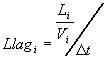
Dflow is the diversion which is zero in this case. Li is the length
of river section i, vi is the average flow velocity on river section
i (m/s), and t is the time step.
Piezometric heads and flows are calculated using a map-based groundwater flow model that applies simultaneously Darcy's law and the continuity equation. The program also provides graphic display of the calculated values in the form of arrows that represent flow direction and magnitude, and of numbers that represent piezometric heads. Calculated and observed values are then compared.
The volumetric flux in a porous medium can be found using Darcy's law, and it is equal to
q=-K(dh/dx)
For a unit width, the volumetric flow rate (Q) = q*h [L^2/T]. Incorporating Darcy's law,
Q = -K(dh/dx) * h (2)
A mass balance for an incremental volume in the x-direction yields,
Q(in) + N*x - Q(out) = (dh/dt)*x (3)
where::
Q(in) is the incoming volumetric flow rate [L^2/T]
Q(out) is the outgoing volumetric flow rate [L^2/T]
N is the uniform recharge rate [L/T]
x is the incremental length [L]
For a differential control volume we get the equation,
d[K*h(dh/dx)]/dx + N = dh/dt (4)
For the steady-state conditions (dh/dt=0), the equation can be solved to obtain a relationship describing piezometric head elevation along the length of the aquifer,
K[h^2-h(0)^2] - N*x[L-x] + K*[x/L][h(0)^2-h(L)^2] = 0 (5)
where:
h is the piezometric head elevation [L]
h(0) is the elevation of the river to the west [L]
h(L) is the elevation of the river to the east [L]
x is the distance along the aquifer from the west river [L]
L is the total length of the aquifer [L]
Differentiating equation (5) with respect to x, and combining it with equation (2), we get,
-Q(x) = K(dh/dx) * h = N(L/2-x) - [K/2] L [h(0)^2-h(L)^2] (6)
in which a positive Q implies that the is flow in the positive x direction. The location of the highest point of the water table can be found by setting dh/dx equal to zero and solving for x,
x = [L/2] - [K/(2*N*L)] [h(0)^2-h(L)^2] (7)
We will now use these equations to predict the response of the groundwater system. Using equation (7), calculate the water levels at points 15 km, 25 km and 35 km along the length of the aquifer. Recall that h(0) = 50 m, h(L) = 50 m, K = 1 m/hr, N = 0.5 mm/day and L = 50 Km. Note that the aquifer water level is the same at 15 km and 35 km. This is a result of having both rivers at the same level.
A script can be run to calculate steady-state conditions. Hydrologic conditions such as fluxplot must be supplied to the script. The results are shown below.
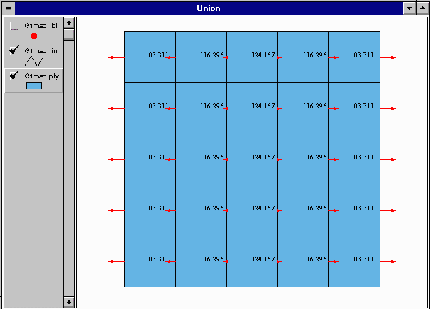
The red vectors represent the magnitude and direction of flow rates across the cell border. The numbers are the piezometric head levels in the center of each of the cells.If one was to calculate using equations (5) and (6), the results would be approximately equal to the results given by the script.
The main goal here is to give an understanding of how ArcView can be applied to study river basin management using the Souss Basin in Morocco as a study example. The project consists of these parts:
1.Use of the USGS 30" digital elevation model as a basis for defining the subwatersheds and stream network of the Souss Basin. This requires Arcview 3.0 and its Spatial Analyst extension. You can skip this part of the exercise if you don't have the Spatial Analyst.
2.Running a set of preprocessor programs to set up the data tables needed to operate the surface water flow simulation program. These tables are prepared for a period of 30 days of daily simulation, from Nov 4 to Dec 3, 1988. This period is selected as a representative example of data from the wetter period of the year in the Souss Basin and is kept short so the exercise can be done reasonably quickly.
3.Interpolating the daily precipitation from point measurement stations to the centroids of each subwatershed using an inverse distance squared algorithm.
4.Running the surface flow simulation program to determine the
flow at a stream gaging station near the outlet of the basin.
The simulation of the Souss basin also needs to account for the presence of three large dams in the basin and for exchange of water between the surface and shallow groundwater systems. Work on these aspects of the model iscontinuing. Without these items included in the surface water simulation, the results are rather approximate. But the intent here is to document how to build a model.
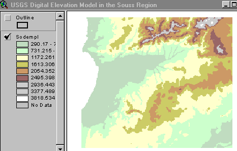
The DEM of Northwest Africa, shown below, is examined.
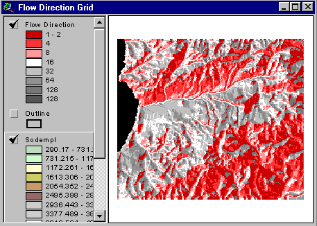
The flow direction grid is calculated by ArcView using the 8-direction pour point method. Each cell in this grid is assigned a value 1, 2, 4, 8, 16, 32, 64, or 128 indicating that the flow direction is in the east, southeast, south, southwest, west, northwest, north, or northeast direction.
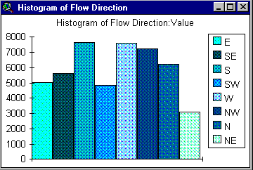
A histogram showing the number of cells in the grid flowing in each direction can be made in the View Menu bar. The principal flow directions are to the South, West and Southwest, reflecting the drainage of water south out of the Atlas mountains and then West to the Atlantic Ocean. There is also a significant flow coming North from the lower mountains forming the Southern boundary of the basin. Close this histogram window in the View.
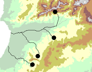
A script is available that traces the flow path of water from any cell in the DEM to the edge of the DEM. The three upper paths shown here all drain to the Souss river, while the fourth path to the South flow through a separate outlet to the ocean, but is included in the study because its drainage area also overlies the Souss aquifer.
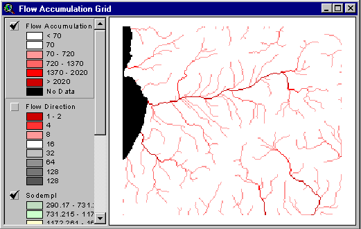

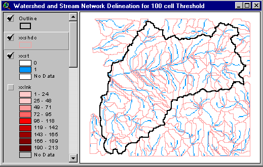
To create a watershed delineation, ArcView runs a program which creates a set of grids. The watershed delineation program uses the logic that a stream is begun whenever the cells have a drainage area greater than the threshold of 100 cells (or 100 sq. km in this case), and a watershed is delineated for each stream link with its outlet cell at the stream junction where this link discharges its water into the next downstream link. Each watershed has a unique grid-code. It is much easier to view the watersheds if they are converted to polygon features. Clicking on the C button, converts the watersheds to polygon features. Here is the result for the 100 cell flow accumulation. Although it is complicated, simpler networks can be created by increasing threshold accumulation.
To simulate water, a series of scripts can be run. These scripts include the following actions:
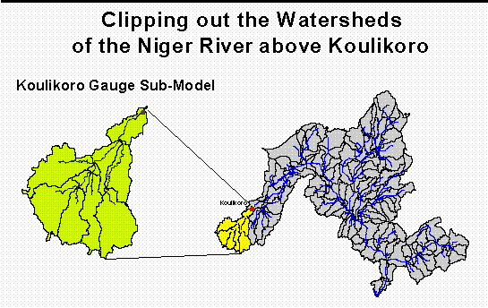
The results presented here are provisional and are subject to change as the project continues. The graphics attached depict the simulated and observed flow for the Niger river at Koulikoro, one of the principal gaging stations on the Niger river above its Inner Delta.
The results are obtained by clipping out a portion of the main basin model to form a Koulikoro submodel, including just those watersheds whose drainage passes through the gage at Koulikoro. Then the model parameters are optimized so that the discharge record there is fitted as well as possible.
The simulations carried out so far are for a 90 month period from July 1983 to December 1990. In the attached flow chart, the horizontal axis is the time in months from July 1983, the vertical axis is the Niger River discharge in cubic meters per second, the green lines are the calculated flows and the red lines are the measured flows at Koulikoro.
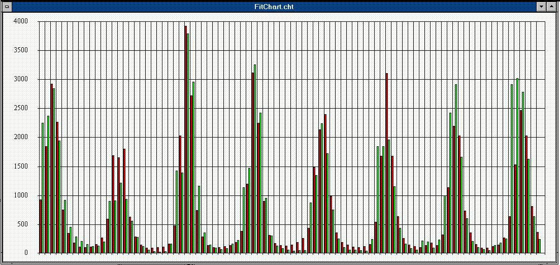
The observed flow data were obtained from the Global Runoff Data Center in Koblenz, Germany.