This exercise is intended for you to build a base map of geographic and flow data for a watershed using the Guadalupe Basin in South Texas as an example. This base map comprises watershed boundaries from the US Geological Survey's Hydrologic Unit Code (HUC) coverage and streams from the US Environmental Protection Agency's River Reach File 1 (RF1) coverage. In addition, you will create a point coverage (shapefile) of stream gage sites by inputting latitude and longitude values for the gages in an ArcView table, creating the shapefile in geographic coordinates, and then projecting it into the same projection as the HUC and RF1 files. You will then link to the US Geological Survey's website in Texas, download some streamflow data and make a plot of the flow hydrograph.
To complete this exercise, you'll need to run ArcView from a PC. If you're really interested, portions of the exercise can be executed in Arc/Info, but it's more tedious. For these instructions, check out Exercise 4 from the 1997 GIS course.
The HUC boundaries are a subdivision of the US made by the US Geological Survey to show major and minor river basins. There are 2-, 4-, 6-, and 8-digit HUC boundaries, where the larger the number the smaller the area. The HUC8 boundaries are the basic ones. I have selected from the maps covering the whole United States, the HUC's and Rf1 reaches in the zone defined by HUC2 = 11, 12 or 13 which is the region covering Texas and neigboring States, and put them into coverages call Huctx and Rf1tx for you to work on. The RF1 coverages have the names of the rivers and streams annotated onto the stream arcs.
The HUC and RF1 coverages for the United States can be downloaded over the internet:
USGS Hydrologic
unit code
EPA river reach
files
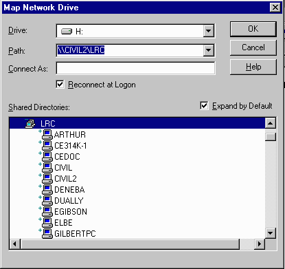
Logon to the computer of your choice and make a directory in your workspace for this exercise. I've saved the needed files in the class directory (Civil2/LRC/Class/Maidment/giswr/basemap/). To be able to access them from ArcView, you'll first need to map the network drive. To do so, open Windows Explorer, and under Tools/Map Network Drive and choose "H:" as the drive, and "\\CIVIL2\LRC" as the path.
The files we'll use are:
edwards.e00, huctx.e00, defgages.ave, and a folder called rf1tx
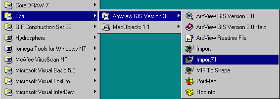
The first two files are in Arc/Info export format, as indicated by the .e00 so you will need to import them using the ArcView Import71 utility.
The Huctx and Rf1tx coverages cover a large region and we only want to work in the Guadalupe Basin. We'll use Arcview to identify which HUC's cover the Guadalupe Basin and to create new Arcview shapefiles of these portions of the coverages.
Start up Arcview.
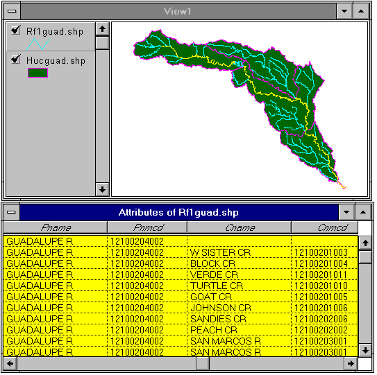
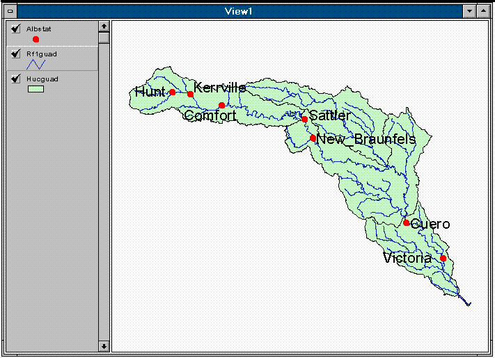
Once Arcview is loaded, open a new view and add the huctx polygon theme to your view. Select (check mark) this theme in your view to get an idea of the scope of this coverage. Recolor the theme as necessary. Highlight the theme by clicking on its legend bar and use the table icon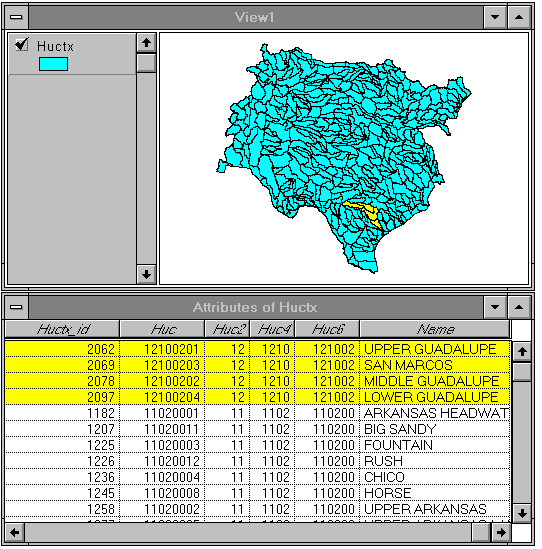 .
.In order to avoid having to work with large data sets which take a long time to draw on the screen, you are going to make a new theme containing only the huc's in the Guadalupe Basin. To do this, highlight the huctx theme in the legend bar, go to Theme/Properties, select the hammer icon, open the Query Builder, build the [huc6] = 121002 query in the same manner as you did previously, except that you select OK in both the Query Builder and Theme Property windows to complete the selection. You'll see that now only the Guadalupe River basin is displayed in the view.
Use Theme/Convert to Shapefile to produce a new theme. Name this theme hucguad.shp and save it in your local workspace for this exercise. You will be prompted to whether add this theme to the View. Do so, adding it to View1 (not New View). If you click on the theme button for hucguad, you'll see that it looks identical to the earlier huctx theme selection for the Guadalupe basin. But the new hucguad shape file is much smaller. A Shapefile is a special simplified file structure for storing geographic features in Arcview. It can be converted to an Arc/Info coverage using the Arc/Info command Shapearc if necessary.
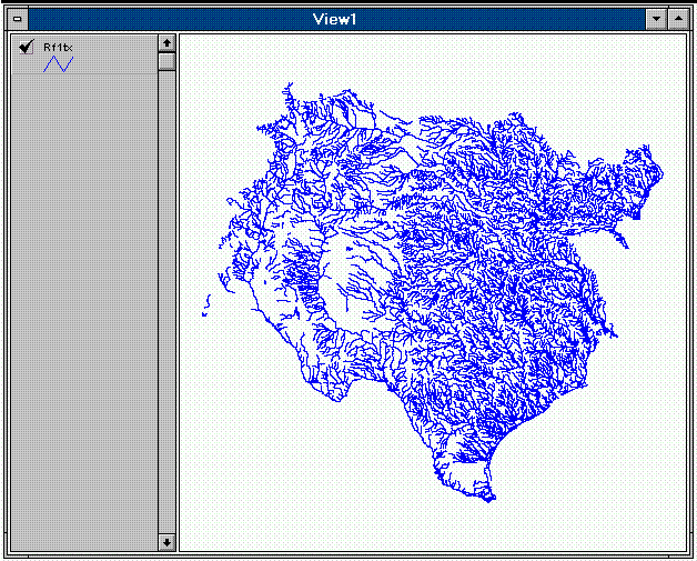
Turn off the huctx and hucguad.shp themes in the View and use the Add
themes button to select a new theme to add to the View. Select rf1tx. Click
this on and you will see a big display of the rivers of Texas and neighboring
states whose drainage comes into Texas.
Highlight the huctx and rf1tx themes in the legend bar (use Shift when highlighting the second theme) and the Edit/Delete Themes to delete them from the Project. From now on, we'll work with the Rf1guad coverage and the Hucguad Shapefiles to save time in displaying the themes.
Once you've got the Guadalupe Basin displayed, you can select the "Zoom
to extent of active themes" button ![]() to bring the Guadalupe Basin up to the full extent of the screen. Now you
should be able to see the Guadalupe River Basin with all of its major river
reaches. If you hit the "i" button with the huctx theme highlighted
and make an information query on one of the huc units, you'll see that
the last field in the attribute table is a "name" field.
to bring the Guadalupe Basin up to the full extent of the screen. Now you
should be able to see the Guadalupe River Basin with all of its major river
reaches. If you hit the "i" button with the huctx theme highlighted
and make an information query on one of the huc units, you'll see that
the last field in the attribute table is a "name" field.
Highlight the rf1guad theme, click on the table icon and bring up the
attribute table for this theme. Scroll across to the names of the rivers.
Pname is the name of the river segment and Cname is the name of the segment
to which this segment next connects downstream. Use the hammer icon in
the Table window to select [pname] = "Guadalupe R", and promote
the selected records to the top of the table. This shows the main channel
of the Guadalupe River. The small gap in the center of the basin is the
segment where the Guadalupe River flows through Canyon Lake, which is separately
identified in the Pname field.
After you've established this view, make a layout of the view and print
it.
To be turned in: the layout of the Guadalupe Basin streams and watersheds..
Now you are going to build a new coverage yourself of stream gage locations on the Guadalupe. I have extracted information from the USGS stream gage data books information about 7 gages on the main stem of the Guadalupe River (there are many other stream gages in this basin):
Seq# Station#   Name         Longitude   Latitude   Mean Annual
                                                     Flow (cfs)
1    08176500  Victoria      97 00 46 W  28 47 34 N     2095

2    08175800  Cuero         97 19 16 W  29 03 57 N     2094

3    08168500  New_Braunfels 98 06 35 W  29 42 53 N      552

4    08167800  Sattler       98 10 47 W  29 51 32 N      464

5    08167000  Comfort       98 53 33 W  29 58 10 N      215

6    08166200  Kerrville     99 09 47 W  30 03 11 N      186

7    08165500  Hunt          99 19 17 W  30 04 11 N       81
The flow data for each of the gages was obtained from the USGS Water-Data Report TX-92-3.
(a) Define a table containing an ID and the long, lat coords of the gages
The coordinate data is in geographic degrees, minutes, & seconds. These values need to be converted to digital degrees, so go ahead and perform that computation for the 7 lon/lat pairs. This is something that you will need to do before going to the computer lab and it has to be done carefully because any errors in conversions will result in the stations lying well away from the Guadalupe River. I suggest that you prepare a table showing the gage long and lat in degrees, minutes and seconds, convert it to long, lat in decimal degrees using the formula
Decimal Degrees (DD) = Degrees + Min/60 + Seconds/3600
Remember that West Longitude is negative in decimal degrees.
To create a new table, go to the project window and double click on the
 icon and click on New. Choose gages.dbf
as the file name and save it in your workspace. You will
see a blank table appear. The table is now in edit mode. Use Edit/Add Field
to create a new field in the Table. In the dialog box that comes up, type
icon and click on New. Choose gages.dbf
as the file name and save it in your workspace. You will
see a blank table appear. The table is now in edit mode. Use Edit/Add Field
to create a new field in the Table. In the dialog box that comes up, type
name Gage No.
type number
width 16
decimal places 0
Click OK and you will see the new field called Gage No. come up in the attribute table. Continue adding fields as follows:
name Latitude
type number
width 16
decimal places 6
name Longitude
type number
width 16
decimal places 6
Once you've done this, go to Table/Stop Editing to save the new fields. If you make a mistake in adding the fields, use Table/Start Editing again and Edit/Delete Field to get rid of the field that you wish to replace. Add a replacement field. It always gets added to the right hand end of the table but you can relocate it in the table by dragging its field name to a new location. Use Table/Save Edits to save the new table fields. It should be noted that a table such as this can be prepared in Excel, saved as a dbf file, and imported into your project using the Add Table button in the project window.
Adding Data to the Table
Use Table/Start Editing and then Edit/Add Record to add a record to the table. Do this seven times to create space for the data on the 7 gages. Now go to the icon bar on the top of the display and select the I button with an arrow on it (just to the right of the I button without an arrow on it).
Go down into the table and you'll see a little hand and finger appear. Use this to click on the record whose value you want to fill in. Now you may enter the data: the gage sequence # (i.e. 1, 2, 3, 4,...) and the longitude & latitude coordinates converted to digital degrees. Continue adding the data values until they are all done.
Example: (this table should contain 7 records, the first one as shown and the other six created similarly by you from the information given above for each gage with the longitude and latitude typed into your file to replace the ... entries given in the table below).
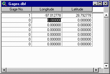
When you are finished, click on any depressed field labels you have to undepress them. Select Table/Stop Editing and save the edits when prompted.
(b) Generate and project a point shapefile showing the gage locations
In order to successfully overlay the stream gage points on top of the RF1 and HUC coverages, they need to be in the same projection as the others. Since the lon/lat values in the gages.dbf table are in decimal degrees, that represents geographic coordinates. We are going to project the points into the Albers Equal-Area Conic projection using an Avenue script developed by Seann Reed. In doing so, we'll also accomplish a datum shift from NAD27 (the datum used for USGS maps from which the latitude and longitude of gages was originally extracted) to NAD83 (the current standard earth datum).
In the project window, double click on the  icon and click the
New button. Select Script/Load Text File. First choose Avenue Script under
List Files of Type: and then select defgages.ave from the class directory
as the file name
and click OK. Before invoking an Avenue script, it must be compiled. Do so
using the
icon and click the
New button. Select Script/Load Text File. First choose Avenue Script under
List Files of Type: and then select defgages.ave from the class directory
as the file name
and click OK. Before invoking an Avenue script, it must be compiled. Do so
using the  icon.
icon.
Using the Window menu, return to your view of the Guadalupe Basin and make sure
it is active (if it's active, there will be a blue bar across the top). Again using the
Window menu, return to script. Be very careful to make sure that you have done both
parts of this step correctly, or an error will occur in the script. Now you can run the script using
the  icon. When prompted, choose gages.dbf as your lat/long table
and choose the appropriate fields. When you reach the Projection Parameters window, it
should lool like this:
icon. When prompted, choose gages.dbf as your lat/long table
and choose the appropriate fields. When you reach the Projection Parameters window, it
should lool like this:
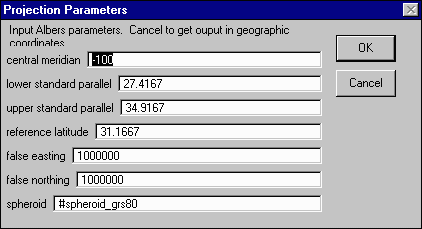
The values shown are the parameters for the Texas State Mapping System in the Albers projection.
Click OK. In the Output Shape File windows, click OK to select your shapefile name
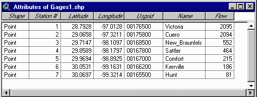
as Gages1. Return to your view window, and the view should now include three themes: Gages1, RF1guad, and Hucguad. Check the Gages1 theme and the USGS stream gage stations will appear. The gage stations from your point
shapefile should fall exactly on the main stem of the Guadalupe River. Pretty cool !!!
This stuff really does work! Use the table icon ![]() to bring up the table of attributes of gages1.shp.
to bring up the table of attributes of gages1.shp.
To be turned in: a screen capture of the gages1.shp attribute table.
Now we are going to add the USGS gage Id, gage name, and annual discharge for
each gage as a new attribute in Arcview. Click on the Table icon in the Project Window and
Select
You will see the new field called Number come up in the attribute table. Continue adding fields as follows:
name USGSID
type string
width 12
Continue adding fields as follows:
name Name
type string
width 16
name Flow
type number
width 8
decimal places 0
Once you've done this, go to Table/Stop Editing to save the new fields. If you make a mistake in adding the fields, use Table/Start Editing again and Edit/Delete Field to get rid of the field that you wish to replace. Add a replacement field. It always gets added to the right hand end of the table but you can relocate it in the table by dragging its field name to a new location. Use Table/Stop Editing to save the new table fields.
Adding Data to the Table
Use Table/Start Editing to begin adding data on the 7 gages. Go to the icon bar on the top of the display and select the I button with an arrow on i, then add the appropriate data value. Continue adding the data values until they are all done.
The following data are needed in the table:
Number    USGSID    Name            Flow

1         08176500  Victoria        2095

2         08175800  Cuero           2094

3         08168500  New_Braunfels   552

4         08167800  Sattler         464

5         08167000  Comfort         215

6         08166200  Kerrville       186

7         08165500  Hunt            81
Click on any depressed field labels you have to undepress them. Then select Table/Stop Editing to close the table. Note that you can only edit tables for which you have write permission (i.e. your own tables not tables in my work area).
Joining the Data Table to the Point Attribute TableGo to the Table icon in the Project Window again, and highlight Attriutes of gages1.shp. Select Add.
Go to the Data table and depress the Number field label. Go to the Attributes Table and depress the Station # field. The order in which you do this is important. There is a one to one relationship between the values in the Number field of the Data table and the Station # field of the Attributes of gages1 table. This is the key field that will be used to join the two tables together.
Use Table/Join to accomplish the Table connection. You will now
have an Attributes of Gages1 table that looks like this:
Now you can use the Name field that you've added as a label for the gages in the View. Go to the View window and under Theme/Properties select the Label symbol. You'll be prompted with a dialog box which permits you to specify what item is to be used as a label. Scroll down to select the Name field. Then use Theme/Auto Label to add the names to the view. You can use Window/Show Tool Palette with the text option to change the size of the labelings. You can use drag the labels around to get a more pleasing arrangement provided the arrow button in the View toolbar is depressed.
You can now create a view like this:
Pretty awesome!
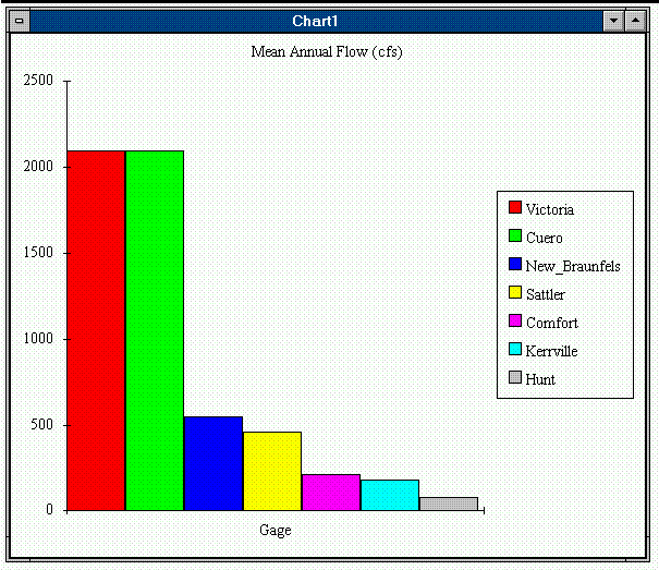
Create a chart of the mean annual flow of the Guadalupe gages by highlighting
the Attributes table, select Table/Chart in the pulldown menus, and in
the dialog box that appears, Add Flow to the display and label the fields
with Name. A bar chart will appear. To edit the title and axes of the chart,
use the small pen tool which is third from the right in the lower tool
bar in the Chart window and then click on the chart feature that you want
to alter.
Prepare a layout showing a map of the drainage area, the graph of its
annual flows at each gage and a table of numerical values describing the
gages. If you add a table or chart and it comes up blank, check that the
Display Always option is used and that the window that you have opened
in the layout is large enough to display the object that is to appear in
it. If necessary resize the original chart or table smaller so that it
can be displayed in the layout. You'll see in the chart that the flow in
the Guadalupe River at Cuero and Victoria is much higher than in the upstream
stations. That is because the flow from the San Marcos river joins the
Guadalupe upstream of Cuero.
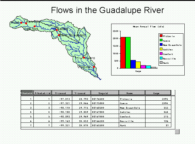
To be turned in: a layout showing the base map, chart and data table for the Guadalupe River flows
The Edwards aquifer is one of the most critical water resources of Central Texas. It is the main source of water supply for San Antonio, the 10th largest city in the United States. The Edwards aquifer is recharged by infiltration from rivers crossing its outcrop area. To determine where the Guadalupe river crosses, the outcrop area, I obtained a coverage of the Edwards aquifer from the Texas Natural Resource Information System by selecting through the menu system: GIS/hydro_geology/major_aqu_e00 where the file edwards.e00 is found. I downloaded this file by logging in to TNRIS using anonymous ftp to: www.twdb.state.tx.us and changing directories to pub/GIS/hydro_geology/major_aqu_e00. Use binary in ftp before downloading files from this area. It seems that you should be able to download this from Netscape but the file displayed on the screen when I did this so I used anonymous ftp to get it directly.
The edwards aquifer coverage from TNRIS is in standard Texas State Mapping System coordinates which are presented in a Lambert Conformal Conic projection. We are using the same coordinates but in an Albers projection because it preserves earth area. I projected the edwards coverage from Lambert to Albers TSMS coordinates using the prj file Lambtsms.prj in the projection library in /res2/maidment/proj. This is the coverage Edwards that you copied from my directory at the beginning of the exercise.
Add the Edwards theme to your Guadalupe project. Click on its legend
and label the theme using the attribute Aquifer. This attribute has three
values: 1 for outcrop, 2 for downdip and 0 for holes within the outer boundary
of the aquifer. Classify the values with Unique Value and color them appropriately.
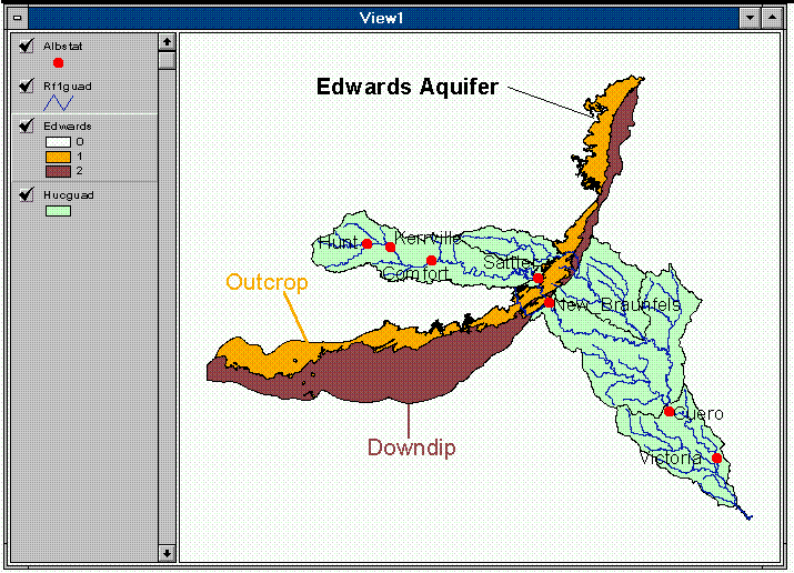
You'll see that the Guadalupe river flows South East towards the Gulf Coast
and it cross first the outcrop and then the downdip portions of the Edwards
aquifer. The downdip region is where the aquifer dips below the land surface
and is shielded from the surface rivers by overlying hydrogeological units
of low permeability. The Edwards is a fissured limestone aquifer whose
fissures lie along its Southwest to Northeast orientation, so its flow
moves in that direction, transverse to the direction of flow in the Guadalupe
basin. It is thus quite possible for water to drain from the Guadalupe
river into the Edwards aquifer and then reappear as a spring further North
in another river, such as Comal springs feeding the Comal river. Zoom in
to the region where the aquifer crosses the Guadalupe basin for a closer
look.
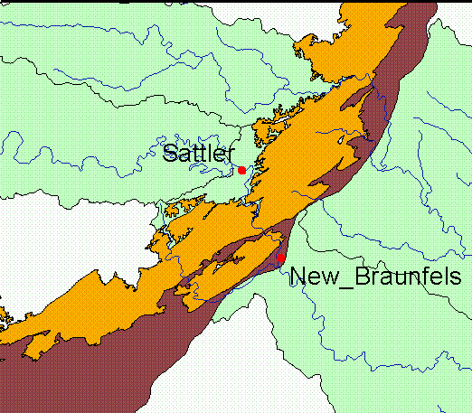
To be turned in: Between which two gaging stations does the Edwards
aquifer outcrop area occur? What is the difference in mean annual flow
at these two gages? Comment on these data. Do they seem correct to you?
There are also other sources of flow data. One of them is via Internet from the U.S. Geological Survey in Texas. To retrieve stream flow data from that site, select the Guadalupe River Basin. You'll then see a list of USGS stations from which you should choose one. I picked Station Number 08176500, the Guadalupe River at Victoria, TX. Go to the "daily-value data archive" link at the top of the page. You now have to specify what data you want to retrieve. Click on the button "Mean" under data type"DISCHARGE, IN CFS" and (near the bottom of the page) specify the time interval. I selected 1/1/91 to 12/31/93 because there was a large flood in South Texas in Christmas of 1992 and I wanted to look at its flow characterstics. It is clear that the first six months of 1992 were a very wet period when compared to the corresponding periods in 1991 and 1993.
Select "Return standard graph", then click on the "Submit"
button (Retrieving the graph may take awhile). Pretty cool!
You can also download data from this source or create graphs for different
time periods. You'll eventually get a plot of Discharge vs. time for your
selected station. My graph looks like this:
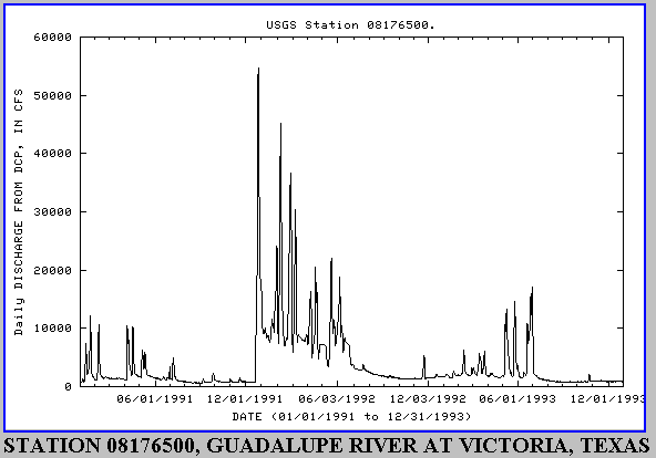
Print your graph from Netscape.
To be turned in: a graph of the discharge from one of the USGS stations on the Guadalupe River.
Ok! You're done!