GIS in Water Resources
Fall 2010
Prepared by David G. Tarboton, David R. Maidment and Saleh
Taghvaeian
Goal
The goal of this exercise is to serve as an introduction to Spatial Analysis with ArcGIS.
Objectives
· Calculate slope from a grid digital elevation model
· Apply model builder geoprocessing capability to program a sequence of ArcGIS functions
· Use raster data and raster calculator functionality to calculate watershed attributes such as mean elevation, mean annual precipitation and runoff ratio.
· Interpolate data values at points to create a spatial field to use in hydrologic calculations
Computer and Data Requirements
To carry out
this exercise, you need to have a computer, which runs the ArcInfo version of ArcGIS 10. The necessary data are provided in the
accompanying zip file, http://www.caee.utexas.edu/prof/maidment/giswr2010/Ex3/Ex3.zip
Readings – at http://help.arcgis.com
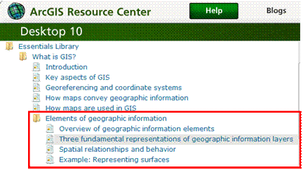
• Elements of geographic information starting from “Overview of geographic information elements” http://help.arcgis.com/en/arcgisdesktop/10.0/help/00v2/00v200000003000000.htm to “Example: Representing surfaces”
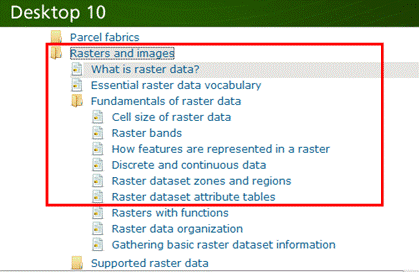
• Rasters and images starting from “What is raster data” http://help.arcgis.com/en/arcgisdesktop/10.0/help/009t/009t00000002000000.htm to end of “Raster dataset attribute tables”
Part 1. Slope calculations
1.1 Hand
Calculations
Given the following grid of elevations. Calculate by hand the slope and aspect (slope direction) at the grid cell labeled A using
(i) The standard ESRI surface slope function (see lecture 7 slides 47-49 in Spatial.ppt)
(ii) The 8 direction pour point model (see lecture 7 slides 50-51 in Spatial.ppt)
Refer to the powerpoint slides (http://www.caee.utexas.edu/prof/maidment/giswr2010/visual/spatial.pptx ) from lecture 7 to obtain the necessary formulas for each of these methods
Grid cell size 100m
|
78 |
84 |
62 |
65 |
65 |
|
81 |
81 |
72
A |
68 |
74 |
|
81 |
110 |
90
B |
83 |
90 |
|
89 |
87 |
80 |
78 |
81 |
Comment on the differences and indicate which you think is a better approximation of the direction of water flow over the surface.
To turn in:
Hand calculations of slope at point A using each of the two methods and
comments on the differences.
1.2 Verifying calculations using ArcGIS
Verify the calculations in (1.1) using ArcGIS Hydrology and Surface Toolbox functions.
Save the following to a text file 'elev.txt' (This file is also included in http://www.engineering.usu.edu/cee/faculty/dtarb/giswr/2010/Ex3.zip)
ncols 5
nrows 4
xllcorner 0
yllcorner 0
cellsize 100
NODATA_value -9999
78 84 62 65 65
81 81 72 68 74
81 110 90 83 90
89 87 80 78 81
This shows how raw grid data can be represented in a format that ArcGIS can import.
Open ArcMap and ArcToolbox. Use the tool Conversion Tools à To Raster à ASCII to Raster to import this grid file into ArcMap. Specify the name of the Output raster as elev.tif and give it a disk location. (Note that the extension specifies the grid file format, .tif for a TIFF file, .img for an ERDAS IMAGINE file, or no extension for an ESRI GRID raster format.) Specify the Output data type as FLOAT (It is more consistent to think of elevation data as including floating point data, rather than integer, even though this specific case is integer data).

You can use the identify button on the grid created to verify that the numbers correspond to the values in the table above.

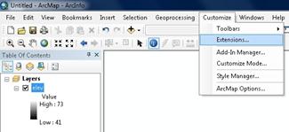
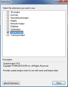
Open Customize à Extensions and verify that the Spatial Analyst function is available and checked. This is where the spatial analyst license is accessed, so if Spatial Analyst does not appear you need to acquire the appropriate license.
|
|
|
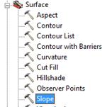
Open the tool Spatial Analyst Tools à
Surface à Slope
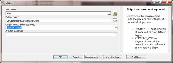
Click on the Show Help>> and Tool Help button to read details on this tool. Note that when you click on each field in the dialog box the help part of the dialog to the right explains the content of the file or option. Select elev as the input raster and specify names for the output raster (e.g. Slope). Note that raster file names cannot exceed 13 characters. Set the Output measurement to PERCENT_RISE and leave the Z factor at 1. Click OK.
The resulting Slope grid should be added to the display. Use identify to verify your hand calculation for grid cell A and note the value of slope for grid cell B.
Open the tool Spatial Analyst Tools à Surface à Aspect. Select elev as the Input raster and specify a name for the output raster (e.g. Aspect). Click OK.

The resulting Aspect grid should be computed and added to the display. Use identify to verify your hand calculation for grid cell A and note the value of aspect for grid cell B.
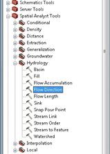
Open the tool Spatial Analyst Tools à Hydrology à Flow Direction
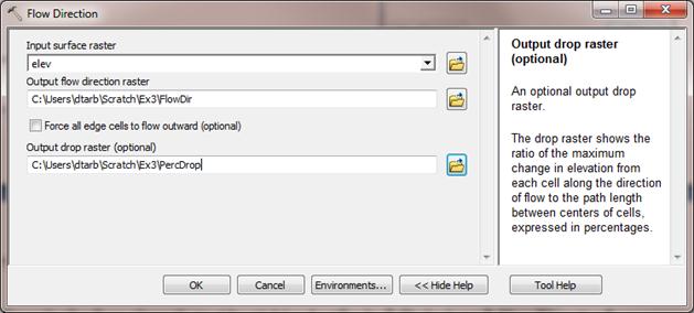
Select elev as the input raster and specify names for output rasters (e.g. FlowDir and PercDrop). Note that the help explanation that appears when click on the output drop raster field in the dialog box explains that the Output drop raster is really the slope expressed as a percentage. Click OK
Use the identify button on the FlowDir and PercDrop grids that are created to verify that the numbers correspond to the values you calculated by hand and resolve or reconcile any differences. Record in a table the ArcGIS calculated flow direction and hydrologic slope (Output drop) at grid cells A and B.
TauDEM Extra for USU students (and others
who have computers where TauDEM can be installed).
[Texas and Nebraska students without access to TauDEM can skip this section. However if you are using a computer where you have System Administrator permissions and can install TauDEM, you are encouraged to try it.]
The D¥ algorithm is not part of standard ArcGIS. Rather it is part of TauDEM that is available from http://hydrology.usu.edu/taudem/. TauDEM should already be installed on the USU computers in the ENGR 305 PC lab used for this class, however if you are working elsewhere you need to download and install TauDEM version 5. Installation requires System Administrator permissions. The installation procedure is a little bit complicated as TauDEM uses a parallel processing package called MPICH2. The installation steps on the website (http://hydrology.neng.usu.edu/taudem/taudem5.0/installation.html) need to be followed exactly for this to work. Also although TauDEM does have a graphical user interface developed for earlier versions of ArcGIS, this does not work for ArcGIS 10. Therefore to use TauDEM in ArcGIS 10 you need to run it from a command line, or from some Python Scripts I have provided that are in Ex3\TauDEMDinfTools. The Python Scripts are easiest, so this exercise uses them. However the command line scripts are more powerful and have greater flexibility. You can learn about them from http://hydrology.usu.edu/taudem/taudem5.0/TauDEM5CommandLineGuide.pdf.
Hand Calculation
Given the grid of elevations on page 2, calculate by hand the slope and flow direction at the grid cell labeled A using the D¥ algorithm. Slides 54 and 55 in the exercise 7 lecture give the necessary formulae.
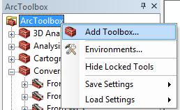
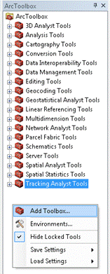
Verify these hand calculations by running the TauDEM D-Infinity Flow Directions tool. To load the TauDEMDinfTools right click in the whitespace within the ArcToolbox window and select Add Toolbox.
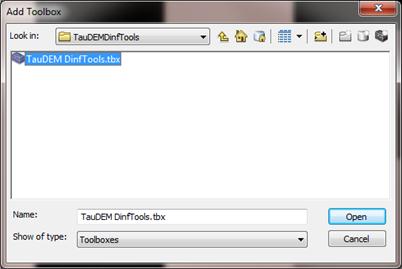
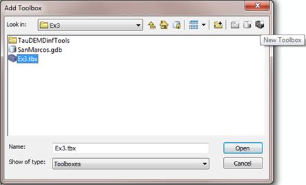
Navigate to Ex3\TauDEMDinfTools\TauDEM DinfTools.tbx and click Open
You should see TauDEMDinfTools in your list of Tools. Click the + to expand and see the tools.
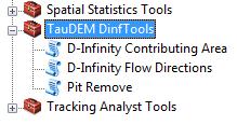
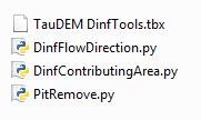
Each of these tools is a Python Script. These are simple python programs that are actually stored in the text files in the folder alongside the TauDEM DinfTools.tbx file.
If you are curious you can use a text editor or right click on Edit to look at these

Double click on TauDEM DinfTools à D-Infinity Flow Directions. This is the function that computes slope and flow direction using the D¥ method. At the dialog box that appears click on the folder browse button next to the Input Pit Filled Elevation Grid and browse to the file elev.tif. TauDEM only works with GeoTIFF format files which was why .tif was used when the elevation data was imported from ASCII. Click on the other browse buttons to fill in output names (e.g. dinfdir.tif and dinfslp.tif, being careful to use the .tif in the file names). Click OK. This is the only TauDEM function needed for this exercise. We may use other TauDEM functions later in the class.
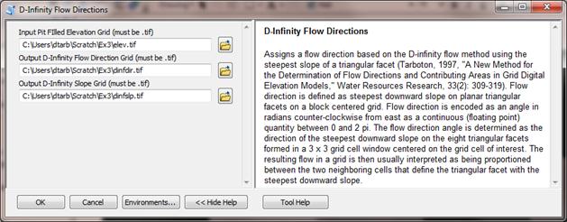
Use the identify button on the dinfdir.tif and dinfslp.tif grids that are created to verify that the numbers correspond to the values you calculated by hand and resolve or reconcile any differences. Record in a table the TauDEM calculated dinfdir and dinfslp at grid cells A and B. Note that TauDEM does not compute values for the edges of the domain, because results there are ambiguous due to the data outside the domain not being present, so TauDEM grids will appear smaller. This is not an error.
End of TauDEM specific work.
To turn in:
Table giving slope, aspect, hydrologic slope and flow direction at grid
cells A and B. If you did the TauDEM
calculations please also include D¥ slope and flow
direction. Please turn in a diagram or
sketch that defines or indicates what each of these numbers means for the
specific values obtained for cells A and B.
1.3 Automating procedures
using Modelbuilder.
Modelbuilder provides a convenient way to automate and combine together geoprocessing tools in ArcToolbox. Here we will develop a Modelbuilder tool to automate the importing of the ASCII grid and calculation of Slope, Aspect, Hydrologic Slope and Flow direction.
Right click on the whitespace within the ArcToolbox window and select Add Toolbox. Navigate to a folder where you want to store your work (e.g. Ex3). In the opened window, click on the New Toolbox icon and name it Ex3.tbx (or something else you might like). Click Open.
|
|
|
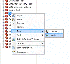
Right-click on the new toolbox and select new model.
The model window should open. This is a window where you can drag, drop and link tools in a visual way much like constructing a flow chart.
In the Toolbox window browse to Conversion Tools à To Raster à ASCII to Raster. Drag this tool onto the model window.
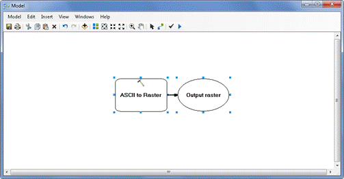
Double click on the ASCII to Raster rectangle to set this tool's inputs and outputs.
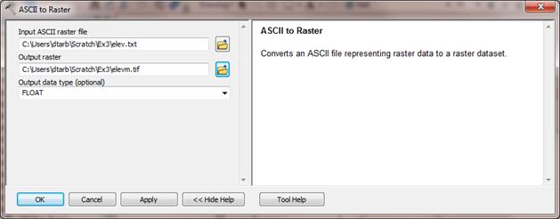
Set the Input ASCII raster file to elev.txt and Output raster to elevm.tif (I used Elevm.tif so as not to conflict with elev.tif that already exists). Set the output data type to be FLOAT. Click OK to dismiss this dialog. Note that the model elements on the ModelBuilder palette are now colored indicating that their inputs are complete.
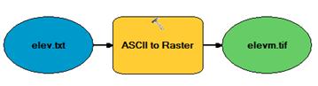
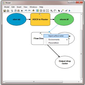
Locate the tool Spatial Analyst Tools à Hydrology à Flow Direction and drag it on to your window. Your window should appear as follows.
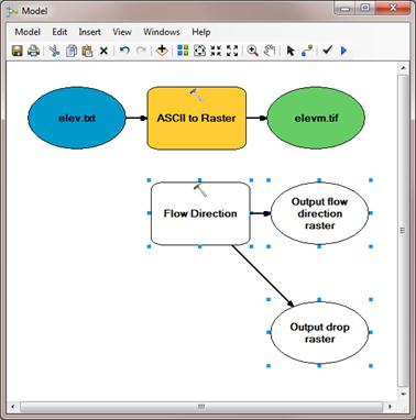
The output from the
ASCII to raster function needs to be taken as input to the Flow Direction
function. To do this use the connection
tool ![]() and draw a line from elevm.tif, the Output raster of ASCII to Raster, to Flow Direction. At the dialog that pops up select Input surface raster to indicate that
elevm.tif is to be used as the input Surface raster for the Flow Direction
tool.
and draw a line from elevm.tif, the Output raster of ASCII to Raster, to Flow Direction. At the dialog that pops up select Input surface raster to indicate that
elevm.tif is to be used as the input Surface raster for the Flow Direction
tool.
Notice that the "output drop" oval is hollow. This is because this is an optional output that has not been specified. Double click on the Flow Direction tool and specify names for both the Output flow direction raster and optional Output drop raster.

Click OK. Alternatively you could double click on output
ovals individually to specify the output rasters. The model is now ready to run. Run the model by clicking on the run button![]() .
.
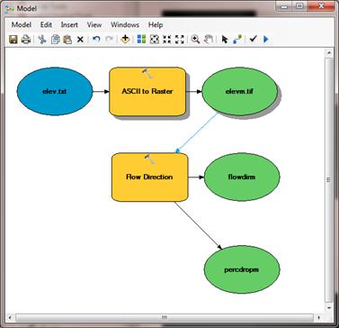
The orange boxes briefly flash red as each step is executed. The Model progress box opens and the progress bar indicates when the model completes. You can then add the outputs to the map and examine the results.
In the model, use
the layout tool ![]() to organize the layout.
to organize the layout.
Add the Spatial Analyst à Surface à Slope tool to your model by dragging it onto the model window. Connect the elevm.tif output to this tool, specifying that it is the Input Raster for the Slope Tool.

Add the Spatial Analyst à Surface à Aspect tool to your model connecting it to elevm.tif as an input in a similar way. Double click on the Slope and aspect tool outputs and specify file names for the outputs.
When setting names you need to be careful that you do not use a name of a grid that already exists, or else you will get a yellow warning sign in the display and the model will not run, as shown below:
![]()
Double click on the Slope tool and set the Output measurement to PERCENT_RISE. Your model should appear as follows.
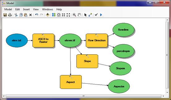
You can click run and do all the processing required to import the data, compute Slope, Aspect, Flow Direction and Hydrologic Slope at the click of a button. Pretty slick!
Right click on elev.txt and select Model Parameter.
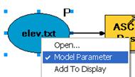
Right click on each of the outputs FlowDirm, percdropm, Slopem and Aspectm in turn and select Model Parameter and Add to Display.
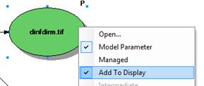
A P now appears next to these elements in the diagram indicating that they are 'parameters' of the model that may be adjusted at run time. Close your model and click Yes at the prompt to save it. Right click on the model in the Toolbox window to rename it something you like (e.g. FlowDirection).
Right click on the whitespace within the ArcToolbox window and select Save Settings à To Default
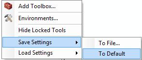
This saves your toolbox settings so that your system remembers the tools you have loaded (in this case the tool you have written in Ex3.tbx). This is useful if you want to not have to hunt for this Toolbox and load it again if you exit from ArcGIS or if there is a crash. This applies to the specific computer you are using so on a shared lab computer it is not really necessary.
If you go back to your model and now double click on it or Open it,
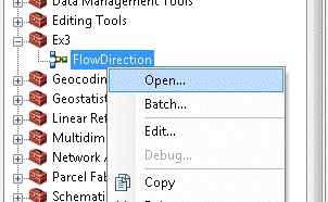
you’ll see that the input files are shown as parameters of the model just like when you execute a tool in ArcToolBox.
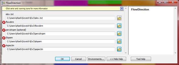
Where you see
warnings or a red X ![]() near one of your files, it usually either
means that there is already a file of that name in the place where you propose
to put the output or there is no input file.
These can be resolved by setting the inputs and outputs correctly.
near one of your files, it usually either
means that there is already a file of that name in the place where you propose
to put the output or there is no input file.
These can be resolved by setting the inputs and outputs correctly.
You are done creating this model. Close ArcMap.
ModelBuilder is a very powerful way of creating complex analyses, and documenting your “workflow” in a form that is visual and can readily be described. In this way, analyses that you’ve done can be passed on to other analysts, and you can also use the visual palette display in your term project report or thesis to document how you’ve done your analysis, so the visual aspect of the display helps with documenting your work, as well as in organizing it.
To turn in:
A screen capture of your final model builder model.
We will now use this model for different data. Reopen ArcMap. Locate the file demo.asc extracted from the zip file of data for this exercise. Double click on your FlowDirection model in the Ex3 toolbox to run it. If you omitted to save settings to default or are on a different computer you will need to add the Ex3 toolbox by right clicking within the toolbox area, selecting Add Toolbox and navigating to where your Ex3.tbx file is on disk. The following dialog box for the tool you created should appear when you open it.

Select as input
under elev.txt the file demo.asc. Specify different names for the outputs to
avoid the conflicts with existing data and remove the red crosses ![]() .
.
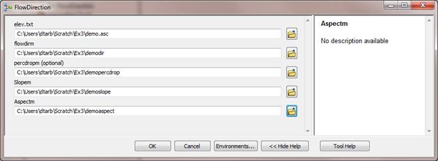
Then click OK and the model should run and add results for this new data to ArcMap. Examine the ArcMap table of contents and record the minimum and maximum values associated with each of the outputs.
To turn in:
A table giving the minimum and maximum values of each of the four
outputs Slope, Aspect, Flow Direction, and Hydrologic Slope (Percentage drop), for
the digital elevation model in demo.asc.
Congratulations, you have just built a Model Builder geoprocessing program and used it to repeat your work for a different (and larger) dataset. If you would like to save this tool to take to another computer or share with someone else you can copy the file Ex3.tbx from its location to a removable media to take with you. If you are going to be sharing this tool more widely there are additional steps to take to clean up the interface (to avoid red X's), label the input fields and document it in help.
Part
2.
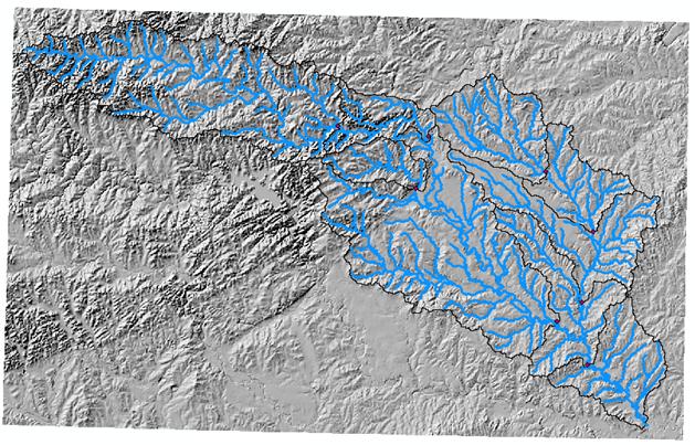
The purpose of this part of the exercise is to calculate average watershed elevation for subwatersheds of the San Marcos basin, and to calculate average precipitation over each of these subwatersheds using different interpolation methods.
The following data is provided in the Ex3.zip file.
SanMarcos.gdb file Geodatabase.
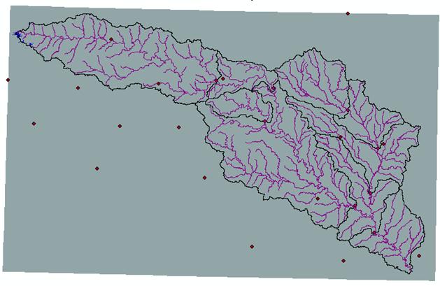
The feature classes Flowline and MonitoringPoint are from Exercise 2. There are two additional feature classes:
- PrecipStn. PrecipStn contains mean annual precipitation data from precipitation stations in and around the San Marcos basin downloaded from NCDC following the procedures given in http://www.ce.utexas.edu/prof/maidment/gradhydro2005/docs/ncdcdata.doc. This data was prepared by downloading all years of available precipitation data for the counties in and around the San Marcos basin, then averaging over these years, retaining only those stations with 6 or more years of annual total data reported by NCDC.
- Subwatershed. Subwatersheds delineated to the outlet of the San Marcos Basin as well as each of the stream gages in MonitoringPoint following the procedures that will be learned in a future exercise.
These new feature classes are in a feature dataset named BaseMapAlbers as it is more sensible to do watershed level analysis where area is involved in a projected coordinate system.
A digital elevation model from the National Elevation dataset is provided in the folder smdem_raw.
1. Loading the Data
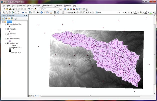
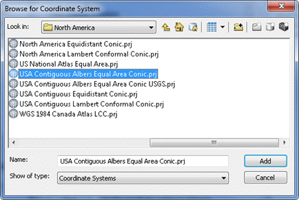
Open ArcMap and from the geodatabase SanMarcos.gdb load the Basemap and BaseMapAlbers feature datasets. Check the coordinate system of each by right clicking and selecting properties. Check the spatial reference system of the data frame layers and if necessary set it to be the same as the BaseMapAlbers feature dataset, "NAD_1983_Albers". We will use this specific NAD_1983_Albers projection, which is the USA Contiguous Albers Equal Area Conic projection, for this exercise.
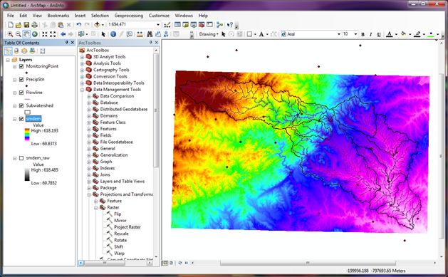
Add the grid smdem_raw to ArcMap. This is a digital elevation model that was downloaded from the USGS seamless data server http://seamless.usgs.gov. Your map should look similar to the following:
The DEM grid is skewed in this display because it was obtained in geographic coordinates. Right click on the smdem_raw layer in the table of contents and select properties. Click on the source tab. This shows you the Cell Size and number of columns and rows. If you scroll down in the properties you also see the Extent and Spatial reference of this DEM.
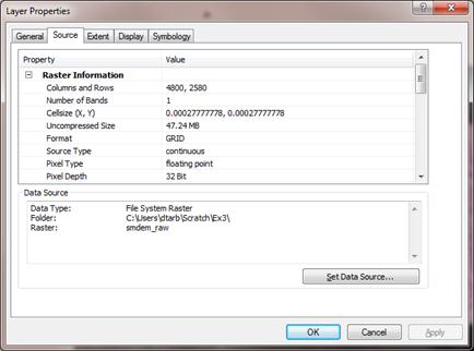
The cell size is in degrees. This is not a very useful measure at this scale. Use what you learned in the lecture on Geodesy to calculate the cell size in m in both the E-W and N-S directions, assuming a spherical earth with radius 6370 km.
To turn in: The number of
columns and rows, cell size in the E-W and N-S directions in m, extent (in
degrees) and spatial reference information for the San Marcos elevation dataset
DEM 'smdem_raw'.
2. Projecting the DEM.
To perform slope and contributing area calculations we need to work with this DEM projected into the Albers equal area projection (An equal area projection is most appropriate for area calculations such as we will be performing). Open the Toolbox and open the tool Data Management Tools à Projections and Transformations à Raster à Project Raster. Set the inputs as follows:

The output coordinate system should be specified using Select a predefined coordinate system … after clicking on the button to the right of Output coordinate system. Then browse to the USA Contiguous Albers Equal Area Conic projection in the Projected Coordinate Systems\Continental\North America folder.
The cell size should be specified as 100 m and CUBIC interpolation used. I have found cubic interpolation to be preferable to nearest neighbor interpolation for continuous datasets such as DEMs. (This NED data is at 1 arc second spacing which is close to 30 m, so in general 30 m would be a better choice here, but 100 m is chosen to reduce the size of the resulting grid and speed data processing and analysis.) CUBIC refers to the cubic convolution method that determines the new cell value by fitting a smooth curve through the surrounding points. This works best for a continuous surface like topography at limiting artificial "striping" that can appear in a shaded relief map (we will construct a shaded relief map below) with the other methods. Click "OK" to invoke the tool. After the process is complete, the projected DEM, smdem, is added to ArcMap.
Examine the properties of the projected dataset.
To turn in: The number of
columns and rows in the projected DEM.
The minimum and maximum elevations in the projected DEM. Explain why the minimum and maximum
elevations are different from the minimum and maximum elevations in the
original DEM.
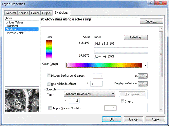
The spatial information about the DEM can be found by right clicking on the smdem layer, then clicking on PropertiesàSource. Similarly, the symbology of the DEM can be changed by right clicking on the layer, PropertiesàSymbology.
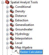
To explore the highest elevation areas in your DEM select Spatial Analyst Tools à Map Algebra à Raster Calculator.
Double click on the layer smdem with the DEM for San Marcos. Click on the “>” symbol and select a number less than the maximum elevation. This arithmetic raster operation will select all cells with values above the defined threshold. In the example below a threshold of 600m was used.
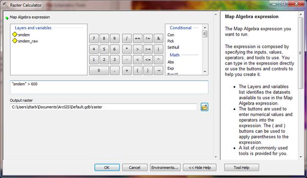
A new layer called raster appears on your map. The majority of the map (grey color in the figure below) has a 0 value representing false (values below the threshold), and the blue region has a value of 1 representing true (elevations higher than 600 meters).
Zoom in to the
region of highest elevations (red region) and do some sampling on the smdem
grid using the identify ![]() tool or pixel inspector
tool or pixel inspector ![]() to identify the grid cell of maximum
elevation. Use the draw tools to mark your
point of maximum elevation and label it with the elevation value for that
pixel.
to identify the grid cell of maximum
elevation. Use the draw tools to mark your
point of maximum elevation and label it with the elevation value for that
pixel.
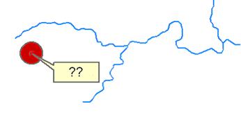
To turn in: A layout showing the
location of the highest elevation value in the San Marcos DEM. Include a scale bar and north arrow in the
layout.
4. Contours and Hillshade
Contours are a useful way to visualize topography. Select Spatial Analyst Tools à Surface à Contour. Select the inputs as follows:

A layer is generated
with the topographic contours for San Marcos. Notice the big difference in
Terrain Relief to the west of the basin compared to the east. This results from
the fact that the Balcones fault zone runs through the middle of this basin, to
the west of which lies the rolling
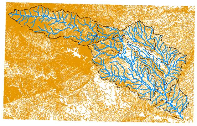
Another option to provide a nice visualization of topography is Hillshading.
Select Spatial Analyst Tools à Surface à Hillshade and set the factor Z to a higher value to get a dramatic effect and leave the other parameters at their defaults (the following hillshade is produced with a Z factor of 10). Click OK. You should see an illuminated hillshaded view of the topography.
To turn in: A layout with a depiction of topography
either with elevation, contour or hillshade in nice colors. Include the streams
from the San Marcos Basemap Flowline feature class and sub-watersheds from the
Sub-Watersheds feature class.
5. Zonal Average Calculations
In hydrology it is often necessary to obtain average properties over watersheds or subwatersheds. The Zonal functions in Spatial Analyst are useful for this purpose.
Select Spatial Analyst à Zonal à Zonal Statistics as Table. Set the inputs as follows:
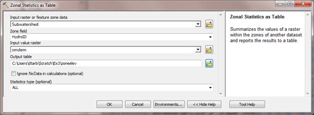
Click OK. A table with zonal statistics is evaluated.
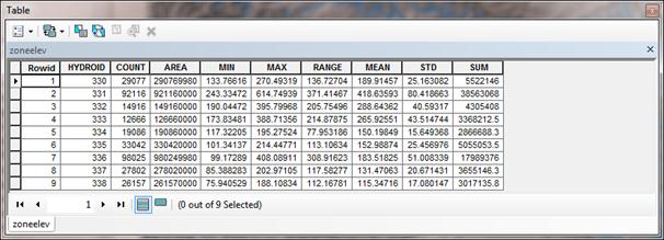
This contains statistics of the value raster, in this case elevation from smdem over the zones defined by the polygon feature class Subwatershed. The Value field in this zone table contains the HydroID from the subwatershed layer and may be used to join these values with attributes of the Subwatershed feature class.
Right click on Subwatershed and select Joins and Relates à Join.
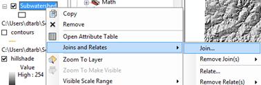
Select HydroID as the field to base the join on and zoneelev as the table to join.
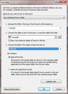
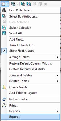
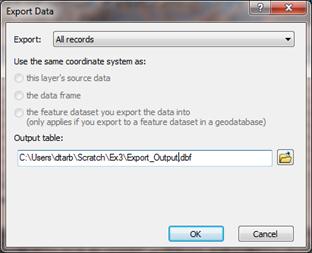
Open the Subwatershed attribute table. Under table options select Export and specify a dbf file for the output.
|
|
|
The exported dbf file can be opened in Excel to examine and present the results. Determine the mean elevation and elevation range of each subwatershed in the SanMarcos Subwatershed feature class.
To turn in: A table giving the HydroID, Name, mean
elevation, and elevation range for each subwatershed in the SanMarcos
Subwatershed feature class. Which
subwatershed has the highest mean elevation?
Which subwatershed has the largest elevation range?
6. Calculation of Area Average Precipitation using Thiessen Polygons
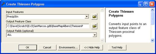
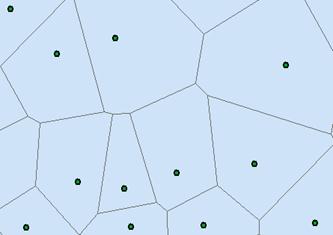
Now to do something really useful. We will calculate the area average mean annual precipitation over the watershed using Thiessen polygons. Thiessen polygons associate each point in a watershed with the nearest raingage. Select the tool Analysis Tools à Proximity à Create Thiessen Polygons

Specify PrecipStn as the Input Features. Set the output feature class to be ThiessenP (saving it in the BaseMapAlbers feature dataset) and indicate that ALL fields should be output. Click OK.
The result is a Thiessen polygon shapefile.
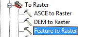
To average precipitation values in these polygons over the subwatersheds we need to convert this to a grid. Select the tool Conversion Tools à To Raster à Features to Raster.
Specify the Input feature as ThiessenP, field as AnnPrecip_in (it is the annual rainfall that we would like to work with), output raster as thiessen and cell size as 100 m. Click OK.
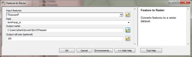
The result should be a grid that gives in each cell the annual precipitation value from the corresponding Thiessen polygon.
Select Spatial Analyst à Zonal à Zonal Statistics as Table. Set the inputs as follows:

Click OK. A table with zonal statistics is created. This contains statistics of the value raster, in this case mean annual precipitation from thiessen over the zones defined by the polygon feature class Subwatershed. The HydroID in this table may be used to join it to the attribute table for the Subwatershed feature class. As for the elevations above this joined table can be exported and examined and presented in Excel.
To turn in: A table giving the HydroID, Name, and mean
precipitation by the Thiessen method for each subwatershed in the SanMarcos
Subwatershed feature class. Which
subwatershed has the highest mean precipitation?
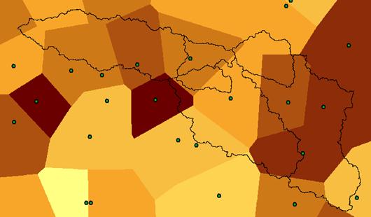
7. Estimate basin average mean annual precipitation using Spatial Interpolation/Surface fitting.
Thiessen polygons were effectively a way of defining a field based on discrete data, by associating with each point the precipitation at the nearest gage. This is probably the simplest and least sophisticated form of spatial interpolation. ArcGIS provides other spatial interpolation capabilities in the Interpolation toolbox in Spatial Analyst Tools.

We will not, in this exercise, concern ourselves too much with the theory behind each of these methods. You should however be aware that there is a lot of statistical theory on the subject of interpolation, which is an active area of research. This theory should be considered before practical use of these methods.
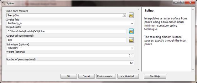
Select Spatial Analyst Tools à Interpolation à Spline. Use the input points from "PrecipStn" and Z value field as " AnnPrecip_in", and set the spline type as Tension with default parameters as follows:
The result is illustrated:
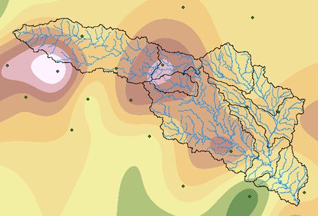
Use Zonal Statistics as Table as before to determine the mean precipitation for each subwatershed in the SanMarcos Subwatershed feature class from the tension spline interpolation.
To turn in: A table giving the HydroID, Name, and mean
precipitation by the Tension Spline method for each subwatershed in the
SanMarcos Subwatershed feature class.
Which subwatershed has the highest mean precipitation using a Tension
Spline interpolation?
Experiment with some (at least one) of the other methods available (Natural Neighbor, Kriging, Inverse distance weighting) to see if you like them.
To turn in. A layout giving a
nicely colored map of the interpolated mean annual precipitation surface over the
San Marcos Basin for one of the methods used and a table showing the mean
annual precipitation for the same method in each Subwatershed. Report what method you used.
8. Runoff Coefficients.
Runoff ratio, defined as the fraction of precipitation that becomes streamflow at a subbasin outlet is a useful measure in quantifying the hydrology of a watershed. Mathematically runoff ratio is defined as
w = Q/P
where Q is streamflow, and P is precipitation. In this formula, P and Q need to be in consistent units such as depth per unit area or volume. In exercise 2 we analyzed the average streamflow at the eight monitoring points in the San Marcos watershed. The flow field in the Monitoring point dataset gives this data, in ft3/s. To convert these to volume units (say ft3) they should be multiplied by the number of seconds in a year (60 x 60 x 24 x 365.25). In the current exercise mean annual precipitation has been evaluated for each subwatershed, in inches. To convert these to volume units (say ft3) these quantities should be multiplied by 1/12 ft in-1 and multiplied by the subwatershed area in ft2. The subwatershed feature class includes subwatershed area, in the units of the spatial reference frame being used, which are m2. (Remember, 1 ft = 0.3048 m). The necessary calculations are most easily performed in Excel. Use the Options/Export function to export the subwatershed featureclass attribute table that includes your Thiessen basin average subwatershed precipitation results to dbf format that can be read by Excel, as was done above. Similarly export the Monitoring Point featureclass attribute table that includes mean annual streamflow at each monitoring point. In Excel multiply gage streamflow by 60 x 60 x 24 x 365.25 to obtain streamflow volume, Q, in ft3. Multiply subwatershed average precipitation (in inches) by subwatershed area (in m2)/(12 x 0.30482) to obtain subwatershed precipitation volume, P, in ft3. On the maps you have that show subwatersheds and streams identify the subwatersheds upstream of each gauge. Add up the precipitation volumes over these subwatersheds then divide Q/P to obtain an estimate of runoff ratio for the watershed upstream of each stream gage.
To turn in. A table giving runoff
ratio for the watershed upstream of each stream gage.
Summary of Items to turn in:
1. Hand calculations of slope at point A using
each of the two methods and comments on the differences.
2. Table giving slope, aspect, hydrologic slope
and flow direction at grid cells A and B.
If you did the TauDEM calculations please also include D¥ slope and flow direction. Please turn in a diagram or sketch that
defines or indicates what each of these numbers means for the specific values
obtained for cells A and B.
3. A screen capture of your final model builder
model.
4. A table giving the minimum and maximum values
of each of the four outputs Slope, Aspect, Flow Direction, and Hydrologic Slope
(Percentage drop), for the digital elevation model in demo.asc.
5. The number of columns and rows, cell size in
the E-W and N-S directions in m, extent (in degrees) and spatial reference
information for the
6. The number of columns and rows in the
projected DEM. The minimum and maximum
elevations in the projected DEM. Explain
why the minimum and maximum elevations are different from the minimum and
maximum elevations in the original DEM.
7. A layout showing the location of the highest
elevation value in the San Marcos DEM.
Include a scale bar and north arrow in the layout.
8. A
layout with a depiction of topography either with elevation, contour or
hillshade in nice colors. Include the streams from the San Marcos Basemap
Flowline feature class and sub-watersheds from the Sub-Watersheds feature
class.
9. A table giving
the HydroID, Name, mean elevation, and elevation range for each subwatershed in
the SanMarcos Subwatershed feature class.
Which subwatershed has the highest mean elevation? Which subwatershed has the largest elevation
range?
10. A table giving
the HydroID, Name, and mean precipitation by the Thiessen method for each
subwatershed in the SanMarcos Subwatershed feature class. Which subwatershed has the highest mean
precipitation?
11. A table giving
the HydroID, Name, and mean precipitation by the Tension Spline method for each
subwatershed in the SanMarcos Subwatershed feature class. Which subwatershed has the highest mean
precipitation using a Tension Spline interpolation?
12. A layout giving a nicely colored map of the
interpolated mean annual precipitation surface over the San Marcos Basin for
one of the methods used and a table showing the mean annual precipitation for
the same method in each Subwatershed.
Report what method you used.
13. A table giving runoff ratio for the watershed
upstream of each stream gage.