Building an Arc Hydro with
Time Series Geodatabase
Prepared by Tyler L. Jantzen, David R. Maidment
and Ernest To
GIS in Water Resources
Fall 2006
Goal
The goal of this exercise is to build a geodatabase for the
Overview
of what is to be done
1.� How to populate an Arc Hydro geodatabase with
spatial and temporal information for a particular river basin.
2.� Show examples of vector-based analysis
available in ArcGIS software for hydrologic data.� Specifically, we will introduce the Utility
Network Analyst and TrackingAnalyst extensions.
4.� Calculate average soil parameters of a watershed
using Spatial Analyst.
3.� Use the Weather Downloader tool to import precipitation
and stream gage flow data into ArcGIS, and animate using TrackingAnalyst.
Computer and Data Requirements
To
carry out this exercise, you need to have a computer, which runs the ArcInfo version of ArcGIS. The data
are provided in the accompanying zip file, http://www.ce.utexas.edu/prof/maidment/giswr2006/Ex6/Ex6Data.zip��
Data description:
Ex6.zip
contains two geodatabases with feature classes that we will use in this
exercise, as well as a raster dataset and XML geodatabase template.� To start this exercise extract the entire
contents of the zip file to a convenient location (e.g. C:\temp\Ex6)
The
contents of the zip file are shown:

The
�SanMarcos_NHDPlus_raw.mdb� geodatabase is the entire
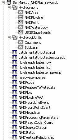
More
information about NHDPlus can be found at http://www.horizon-systems.com/nhdplus/.�
The
second geodatabase, �SanMarcos_ArcHydro_raw� contains some preprocessed files
you will use to create your ArcHydro with Time Series Geodatabase.� Its structure is shown below.
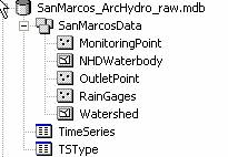
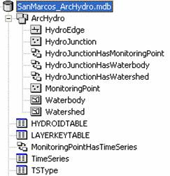
The
SanMarcos_ArcHydro_raw personal geodatabase contains the following
- A feature dataset "SanMarcosData"
that contains the feature classes RainGages,
OutletPoint, MonitoringPoint, Watershed, and NHDWaterbody.
- A table "TimeSeries" that is empty,
but will be filled with data using the Weather Downloader.
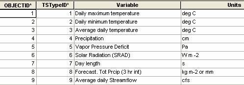
- A table TSType with metadata for the daily rainfall and streamflow
time series records.
The OutletPoint is a point feature marking
the outlet of the
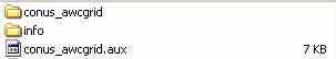
Using
Windows Explorer, the raster file looks like:
Using
ArcCatalog, the same file looks like this:
![]()
The conus_awcgrid is a raster grid of
Average Water Capacity.� This is defined
in the NRCS Soil Survey Manual as "The volume of water that should be
available to plants if the soil, inclusive of rock fragments, were at field
capacity".� The values in this grid
represent the Average Water Capacity as a volumetric percent multiplied by 1000.� This dataset was produced by Doug Miller and
colleagues at
Building an Arc Hydro Geodatabase
In this exercise we will use the Arc Hydro Framework with Time Series schema to build a Arc Hydro geodatabase.� The framework schema provides a simplified version of the full Arc Hydro schema.� There are a number of approaches for building an Arc Hydro geodatabase.� We will take the approach of first creating an empty geodatabase and then loading features into the certain feature classes within the geodatabase.
We will use ArcCatalog to build the geodatabase, so open ArcCatalog.
In your working directory, create a new personal geodatabase and name it SanMarcos_ArcHydro.mdb
Now we are going to apply the Arc Hydro schema to this geodatabase.� The schema is stored in an xml file provided with the exercise documents.� You should be able to see the xml file from ArcCatalog (ArcHydroFrameworkWithTimeSeries.xml).� Double click on the xml file to open the document in a web browser.� Don�t worry if you don�t understand what comes out!
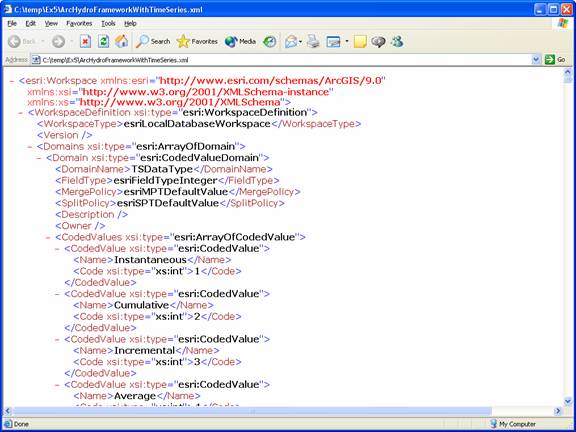
This xml file describes the feature classes, tables, fields, and relationships defined in the Arc Hydro with Time Series schema as depicted in Chapters 2 and 7 of the Arc Hydro book.�
To apply the schema to the empty geodatabase we just created, right-click on the geodatabase and select Import/XML Workspace Document.�

Choose to import only a schema and browse to the ArcHydroFrameworkWithTimeSeries.xml file.�
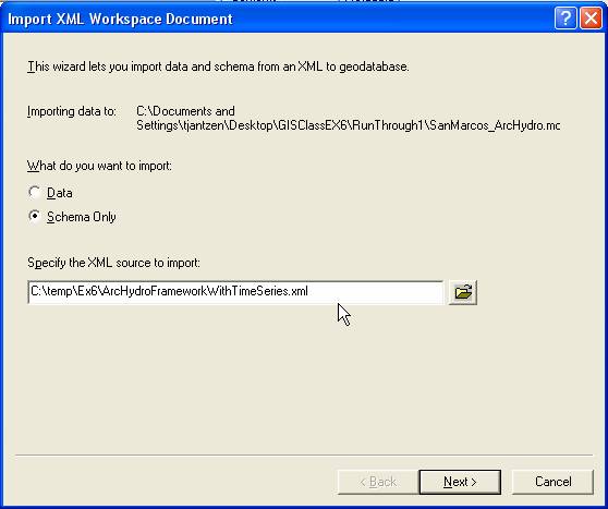
Press Next and then
Finish.
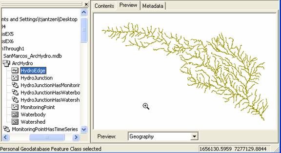
Refresh ArcCatalog (this step is very important or you won�t be able to see your result!) and then look at the SanMarcos_ArcHydro geodatabase.� Notice the structure of the geodatabase.� Preview one of the feature classes�s attribute table (while a feature class is selected, on the right side of ArcCatalog, select the Preview tab.� At the bottom of this tab, choose to preview the table instead of the geography.� You will notice that there are no features in the feature class, but that the feature class has Arc Hydro attributes� (HydroID, HydroCode, etc.).
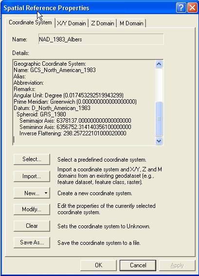
Before we import data, it is smart to first define the coordinate system of the ArcHydro feature dataset.� To do this, we will import the coordinate system of the SanMarcosData feature dataset in the SanMarcosNetwork geodatabase provided with the exercise.�
Right-click on the ArcHydro feature dataset and select Properties, then Edit the spatial reference.� Import the coordinate system of the SanMarcosData feature dataset in the SanMarcos_ArcHydro_Raw geodatabase.� The coordinate system has the following attributes.�� Please note that there was a coordinate system (the USGS National Albers projection) contained in the XML document that you imported to the geodatabase.� We are replacing that with the coordinate system used for the rest of the data (the Texas Centric Mapping System).
 �
�
Ok, now let�s import some data.� One complication is that you are not able to import features into a feature class that is part of a geometric network.� That means we have to break the geometric network, import features into HydroEdge and HydroJunction, and then rebuild the network.
Delete the
HydroNetwork geometric network.� You
can do this by right-clicking and highlighting the HydroNetwork ![]() and pressing
the delete key.
and pressing
the delete key.
We are going to populate the feature classes within our geodatabase by loading data from another feature class.� This is a very useful procedure so it is good to get some practice at using it.
First we are going to load data from the NHDFlowline feature class in the SanMarcos_NHDPlus_raw.mdb geodatabase into the HydroEdge feature class in the SanMarcos_ArcHydro geodatabase.
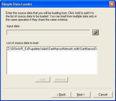
Right-click on the HydroEdge feature class and select Load/Load Data.� (If you see the Load Data button grayed out, it is because you haven�t deleted the HydroNetwork.�� You can�t load data directly into a Network feature class, only to a simple feature class).
Browse to the NHDFlowline feature class within the SanMarcos_NHDPlus_Raw geodatabase (its in the Hydrography feature dataset).� Press Add and then Next.�
Keep the defaults on the next window (you do not want to load the data into a subtype). Press Next.
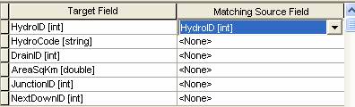
On the next window, make one change.� Set the matching source field for HydroCode to be ComID.� The ComID is a unique identified for NHD reaches, so it makes sense to use this as the HydroCode. Press Next.
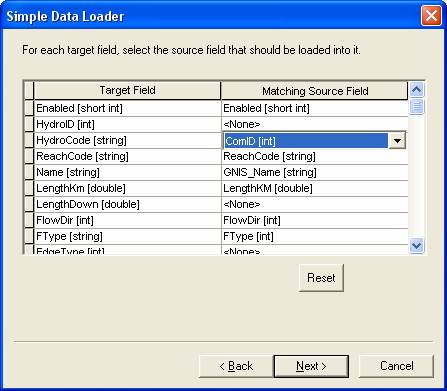
Keep the default on the next window (Load all the source data).� Press Next.
Press Finish to complete the data load.
Once the process has completed, refresh your geodatabase.� You should see the HydroEdge class now populated.
Now let�s do the HydroJunction feature class.� We are going to load two feature classes into HydroJunction: StreamGageAddressPoint and OutletPointAddressPoint.�
First we�ll load
StreamGageAddressPoint.
Right-click on HydroJunction
in the SanMarcos_ArcHydro geodatabase and select Load/Load Data.� ��
Browse to StreamGageAddressPoint in the SanMarcos_ArcHydro_Raw geodatabase.�
Click Add and
then Next.
Match up the fields
as shown below:
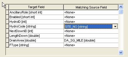
We are using SITE_NO as the HydroJunction�s HydroCode.� This will provide a link between Arc Hydro and data stored outside ArcHydro (like NWIS data) that is referenced to a stream gage by its station number.
Click Next and then Finish to complete the data import.
If you mess up in any of these data loading steps, or inadvertently load the data twice, Open ArcMap, start the Editor and edit out the records or features that you don�t want.
So far so good.� Now let�s add the second feature class to HydroJunction: OutletAddressPoint.�
Right-click on HydroJunction in the SanMarcos_ArcHydro geodatabase and select Load/Load Data.�
Browse to OutletAddressPoint in the SanMarcos_ArcHydro_Raw geodatabase.
Click Add and then Next.
We do not want to transfer any of the fields from Outlet AddressPoint into HydroJunction.
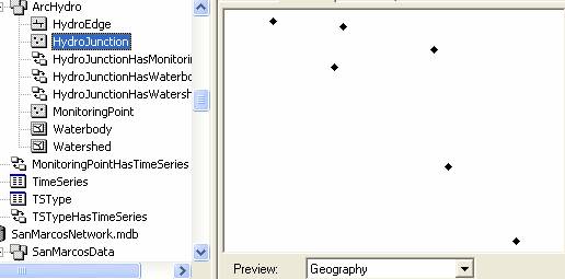
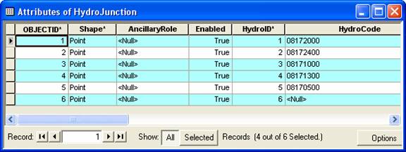
That�s it for HydroJunction.� You should have six features in the feature class now.� Five will be USGS stream flow gages and the sixth the basin outlet.� Its best to check this in the Geographic View since the sixth feature doesn�t seem to show up in the tabular view.
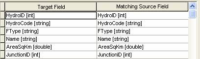
The MonitoringPoint features will come from the MonitoringPoint feature class in the SanMarcos_ArcHydro_Raw geodatabase.� This feature class contains the USGSGage and feature classes and has the proper HydroIDs that link the MonitoringPoints to TimeSeries records.� Some preprocessing of the linkage between the spatial features and time series data has been done here to facilitate you doing this exercise readily.
Follow the same procedure as with the HydroEdge and HydroJunction.�
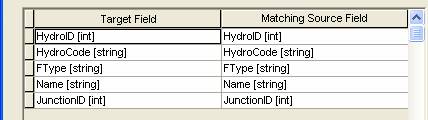
The fields for the MonitoringPoint feature class are:
We are also going to load the Watershed and Waterbody feature classes from the SanMarcos_ArcHydro_raw geodatabase into the Watershed and Waterbody feature classes in the SanMarcos_ArcHydro geodatabase.� Note: we are loading Waterbody (as opposed to NHDWaterbody) because Waterbody has already been preprocessed.
The fields for the Watershed feature class are:
The fields for the Waterbody feature class are:
Finally, we need to load in data from TSType tables.� Load these from the SanMarcos_ArcHydro_raw geodatabase.
The fields for the TSType table are:
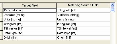
We are doing this so that we�ll know what kind of time series data that we�ll work with later.
That�s it for ArcCatalog.� We have all of our data loaded into our geodatabase.� Next we need to populate some of the attributes in the feature classes.�
Populating Attributes
There are a few key relationships in ArcHydro that we will demonstrate in this exercise.� One is WatershedHasHydroJunction, MonitoringPointHasHydroJunction, and MonitoringPointHasTimeSeries.� To make these relationships functional, we must first populate a few fields within the Watershed, MonitoringPoint, and HydroJunction Feature Classes.
Close ArcCatalog
and open ArcMap.
Add all of the ArcHydro feature dataset and the TimeSeries and TSType tables from SanMarcos_ArcHydro (the geodatabase you just created) to ArcMap.
Add the Arc Hydro Toolbar if you haven�t already.
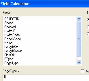
Lets make all the HydroEdges into Flowlines.� Open the Attribute table for HydroEdge and select the attribute EdgeType.� Right Click on it and set its values = 1 as shown below.�� This makes all your edges flow lines as you would wish (as distinct from shorelines around coasts and lakes).
Save your ArcMap document as Ex6Soln.mxd
We are going to give HydroIDs to all of the feature classes, except for MonitoringPoint.� (We aren�t going to give MonitoringPoint features HydroIDs because they already have HydroIDs and are related to TimeSeries records).
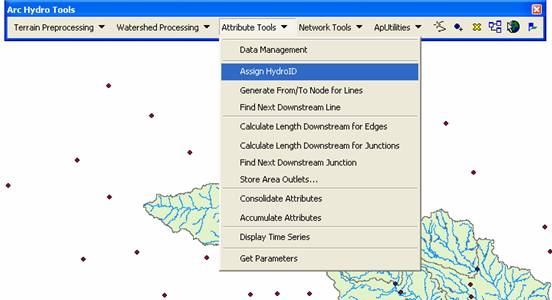
Under Attribute Tools on the Arc Hydro toolbar, select Assign HydroID.
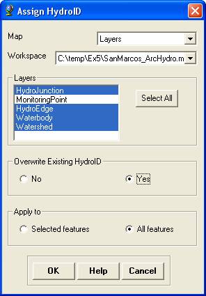
Select all the layers
except for MonitoringPoint.� Choose
to overwrite existing HydroIDs and
to apply the procedure to all features.� Press OK.
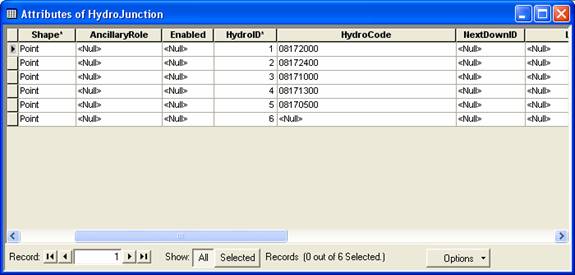
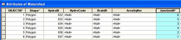
You can see that all of the features now have HydroID populated.� Here�s a look at the HydroJunction feature class:
Now we are going to use the Assign Related Identifier tool ![]() �to link the MonitoringPoint features with
their associated HydroJunction features.�
�to link the MonitoringPoint features with
their associated HydroJunction features.�
Select the ![]() �tool from the Arc Hydro toolbar.� In the pop-up window, choose the source to be HydroJunction�s HydroID and the
target to be MonitoringPoint�s
JunctionID. �Press OK.
�tool from the Arc Hydro toolbar.� In the pop-up window, choose the source to be HydroJunction�s HydroID and the
target to be MonitoringPoint�s
JunctionID. �Press OK.
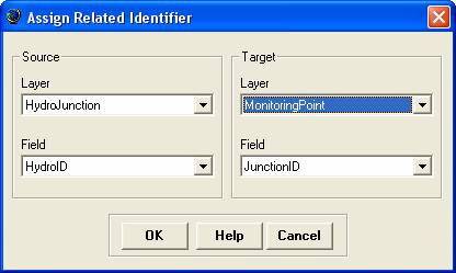
This tool will populate a MonitoringPoint feature�s JunctionID attribute with a HydroJunction�s HydroID, thus establishing a relationship between the two features.
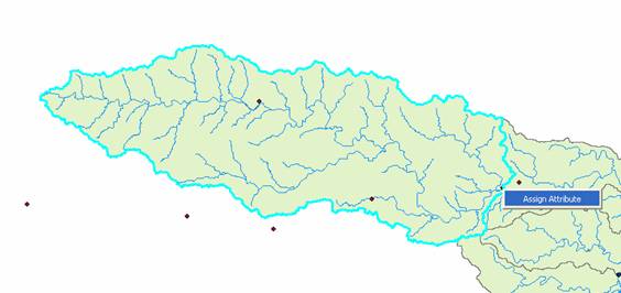
Now, zoom in to one
of the USGS Gage monitoring points, and then select the ![]() �tool again.�
You�ll see the same pop-up menu, but the tool remembers the Target layer
and field we just set so you can press OK.
�tool again.�
You�ll see the same pop-up menu, but the tool remembers the Target layer
and field we just set so you can press OK.
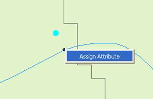
This tool is a little trick to get a handle, so be patient.� First select the MonitoringPoint feature.� Once this is selected, then right-click on the HydroJunction feature.� You should see an Assign Attribute box pop-up.� Click on the Assign Attribute box.� Once you do so, you�ll see both features flash indicating that the MonitoringPoint feature�s JunctionID has been set.�
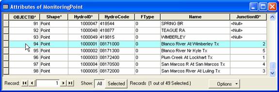
Do this same procedure for the four other MonitoringPoint features.� Note: it may be easiest to select the USGS Gage MonitoringPoint features in the attribute table (as opposed to on the map), and then zoom to the selected feature.� The USGS Gage Monitoring Point features are those with an 8 digit HydroCode.�
If you check the attribute table for Monitoring Points, you�ll see that the JunctionID has been assigned for those MonitoringPoints that are streamgages.
Ok, next we are going to use the same Assign Related Identifier tool to link the Watershed features with their HydroJunction outlet points.� Press the Assign Related Identifier tool and select the target layer to be Watershed and the target field to be JunctionID.� Keep the Source layer and fields as the layer HydroJunction and field HydroID that we set before.
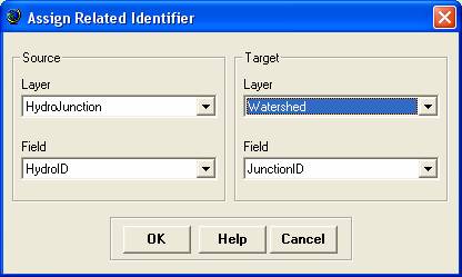
Now, click on a watershed feature, then right-click on its outlet HydroJunction and press Assign Attribute.� Check to make sure the Watershed�s JunctionID is the HydroJunction�s HydroID.�
Follow this same procedure for each of the watersheds, being sure to also include the outlet and most downstream watershed.
Here�s what the attribute table should now look like for the watersheds.
That�s it for data manipulation.� We are now ready to do some analysis.
If you now use the Identify button, you can trace through
the relationships that you have just created.�
Here is how they look for the
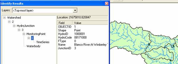
To be turned in:� A screen capture showing the results of an Identify
query for the Watershed, HydroJunction and Monitoring Point for the Blanco
River Near Kyle.
River Networks
Now we�re going to have some fun with the stream lines as a river network.�� Close ArcMap, Open Arc Catalog and examine the SanMarcos_ArcHydro geodatabase.
Right Click on the ArcHydro feature dataset and select New / Geometric Network.� You have to have ArcInfo to complete this task � ArcView does not create networks.��
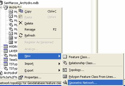
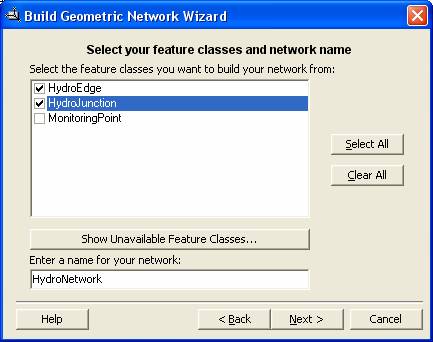
Click Next on the Geometric Network Wizard options until you get to Selecting the feature classes and network name.� Select HydroEdge and HydroJunction as your network feature classes.� Change the network name to HydroNetwork.�
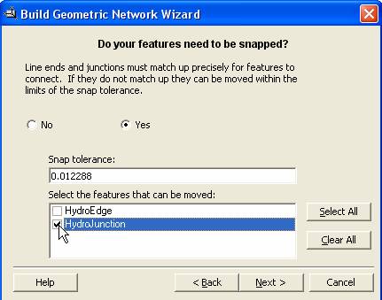
Click Next.� Keep the default of yes to preserve the existing enabled values.� Click Next again.� Change the default, and click yes when it asks if you want complex edges in the network.� Lastly, click yes to snap the features.� The default distance of 0.012288 is fine.� You only need to move the HydroJunction features.� Click Next for all the remaining windows.�
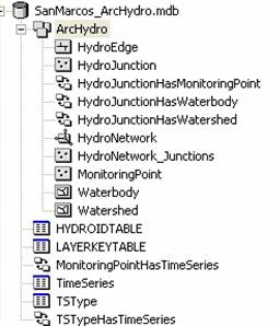
When you finish you�ll see that you�ve created a new geometric network, HydroNetwork, which includes a set of generic network junctions called HydroNetwork_Junctions whose function is to provide geometric connectivity between the HydroEdge features.��
Close ArcCatalog, and open a new ArcMap and add the HydroNetwork to the map.
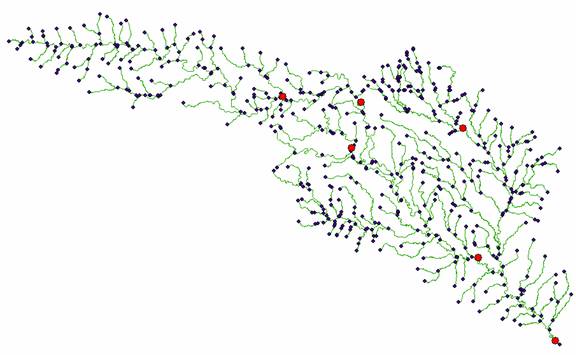
Notice that when you add the network, the HydroEdge, HydroJunction, and HydroNetwork_Junction feature classes are added to the map.� The HydroJunction features which represent MonitoringPoints are now part of the HydroNetwork.� This is be very useful when we do flow tracing, which we are going to do next!
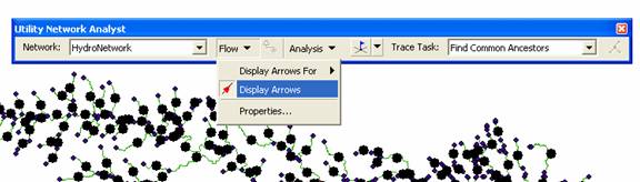
The Utility Network Analyst is an extension to ArcMap for performing analysis with geometric networks. It is called the Utility Network Analyst because geometric networks in ArcGIS are most commonly used in the utility industry, but they are also helpful in water resources research.
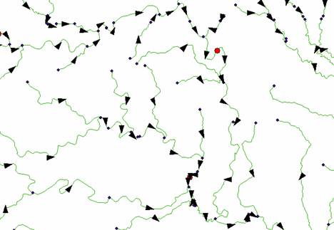
Use View/Toolbars, to display the Utility Network Analyst toolbar and select Flow/Display Arrows.� You�ll see that there are set of * symbols displayed, which means that there is no flow direction set on this network.��
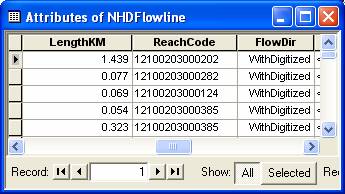
ArcGIS has four possible values for flow direction along a
line: 0 = Uninitialized, 1 = WithDigitized, 2 = AgainstDigitized and 3 =
Indeterminate.�� These values refer to
the direction in which the line has been digitized (as shown by the order of
its vertices).�� Usually, the NHD lines
have been digitized from upstream to downstream, so the flow direction is set
to be WithDigitized.� The NHDinGeo geodatabase design has adopted
this convention from the Arc Hydro design.��
To apply the flow direction attribute values to the network, use the Arc Hydro tools Set Flow Direction (not Store Flow Direction!)
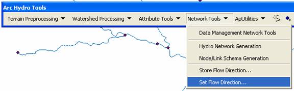
Choose HydroEdge in the Set Flow Direction dialog, Press Ok, and then press the set the flow direction according to the attribute FlowDir. �Note: the following window may appear different than the one shown, depending on your version of ArcHydro.
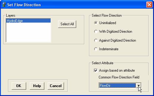
This action takes a couple of minutes as there are 557 Lines to be processed.
Now when we view the flow arrows, they will be pointing in the correct direction.
As you learned in Exercise 5, Open the Utility Network Analyst toolbar, place an Edge flag on a network edge, set the Analysis Options to Select, choose Trace Downstream�
press the Solve button.
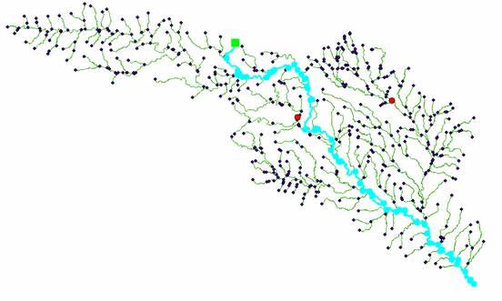
Open the HydroJunction feature class attribute table and notice that four of the six features were selected meaning that these four are downstream of the junction I traced from.� Notice that now your HydroJunctions are participating in the network as well as the edges that you worked with in Ex 5.
We can get the monitoring points related to these features
by selecting Options/Related Tables/HydroJunctionHasMonitoring
Point:Monitoring Point.
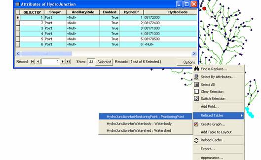
This will bring up the MonitoringPoint attribute table with three of the 6 features selected.� These selected monitoring points are downstream of the junction I traced from.�
To be turned in:� Do a trace from the most upstream junction in
the network and �trace downstream� to the outlet.�� What is the total length (km) of the flow
path thus identified?
How many
HydroJunctions are selected?�� What
stream gages measure flow along this path (give the stream gage names and USGS
ID values).�� What is the total area of
the watersheds that this flow path traverses?
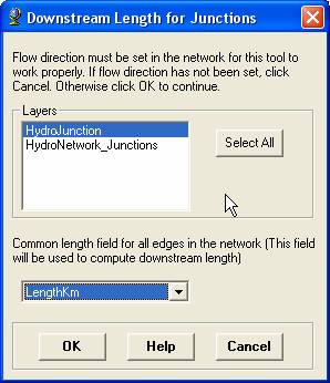
Arc Hydro has some other neat tools for determining network attributes.� One of them finds the Length Downstream for Junctions.� Clear any selected features that resulted from the analysis that you have just done.
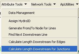
Invoke this tool and select HydroJunctions as the feature class to be processed, and select LengthKm as the field on HydroEdges to be used for the Length calculation
Now if you click on the HydroJunction for the stream gage of
the

and if you navigate through the + signs you can see the gage and the watershed that is relationally linked to this stream gage.
To be turned in:� What is the drainage area of DEM watershed
draining to the gage on the
That�s it for network analysis.� You can see how powerful these tools can be for a complex network where it is not immediately clear what is downstream of what.� This last process of finding the related time series recorded downstream of an arbitrary point on the network is a good segue into our next topic: visualizing space and time in ArcGIS.�
Raster Calculations and
Soils Data
For the next section we will use the watershed areas in conjunction with the Conus Soils data set to determine the Average Water Capacity, averaged over each watershed.� .�
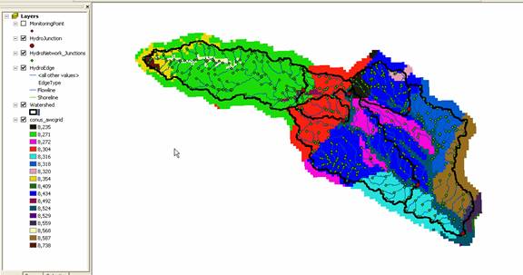
Add the raster conus�_awcgrid from the exercise folder to ArcMap.� Click No when asked to build Pyramids.� The conus_awcgrid has a different projection than the rest of the ArcHydro data we are using, but that should be okay.� Click OK when warned.� Also add the Watershed feature from the SanMarcos_ArcHydro geodatabase.� Your map should now look something like the following:
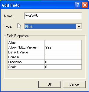
Open the Attributes Table for the Watershed feature class.� Click Options and Add a field �called �AvgAWC.�� Make this field type Float.� This field will store the value we calculate for the average AWC for each watershed.�
Make sure the Spatial Analyst extension of ArcGIS is turned on.� Go to Tools>Extensions and make sure the Spatial Analyst extension is checked.� Also go to View>Toolbars and make sure the Spatial Analyst toolbar is selected.�
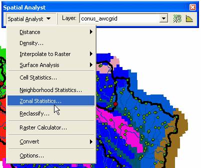
On the Spatial Analyst menu of the Spatial Analyst toolbar, go to Zonal Statistics.�
Use the settings shown in the graphic below for the Zonal Statistics.� For the output table, choose an appropriate path in your exercise folder.�
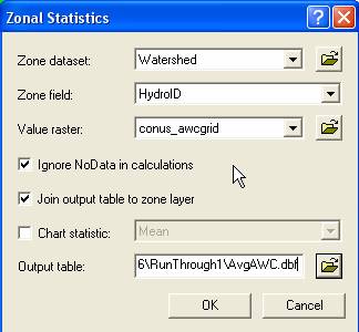
Click OK.� The table that appears is the statistics of conus_awcgird over each of the watershed as defined by the Watershed feature class.� If you open the Attribute Table for the Watershed feature class, you will notice the same values attached to that table.� However, these values are not a permanent part of the Watershed Attribute Table.�
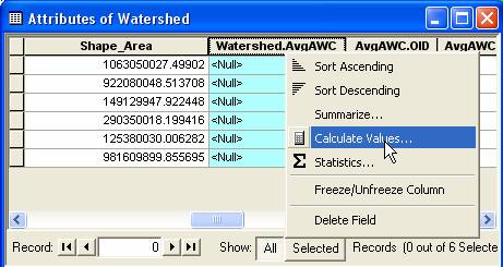
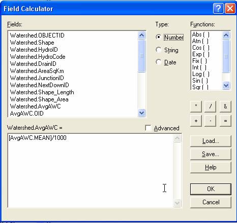
To fill the AvgAWC field of the Watershed Attribute Table, right-click on the Watershed.AvgAWC field and select Calculate Values.�
Click Yes to calculate outside of an edit session.�
Set Watershed.AvgAWC to be equal to AvgAWC.MEAN/1000 by double clicking on AvgAWC.MEAN in the list of available fields.� Dividing by 1000 brings the value to be an actual percent.� Click OK.�
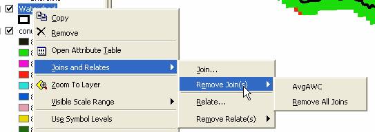
To remove the rest of the zonal statistics from the
Watershed Attribute Table, right-click on the Watershed feature class in the
Table of Contents.� Go to Joins and Relates>Remove Joins>AvgAWC
If you now open the Attribute Table for Watershed, you will notice all the ArcHydro basic information, as well as the Average AWC value for each watershed.�

To be turned in:� A map of the watersheds, symbolized by the quantity of the Average AWC with the value for AvgAWC displayed on the map.��� Also include the Flowlines on this map.�
Adding Temporal Weather Data
In this section we are going to add historical precipitation and streamflow information as a time series for each of the watersheds using web services.� A similar process could be used to download forecasted precipitation, other climatological, or other data that is stored in an Observations Data Model format. �
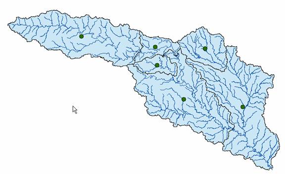
When we download weather data in the next step, we will need a point feature class as the spatial feature from which to add weather data.� Since the outlet point of each watershed is not a good representative location for the entire watershed, we will create a point feature class of the centroid of each of the watersheds.�
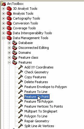
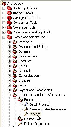
In the ArcMap ArcToolbox browse to and click the tool Data Management
Tools>Features>Feature to Point.� ��
Use the Watershed feature class as the input feature, and title the output feature class WatershedCentroid, saved in the SanMarcos_ArcHydro geodatabase (but not in the Arc Hydro feature dataset because that has a different coordinate system.
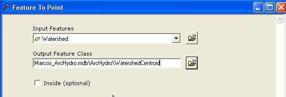
The WatershedCentroid point feature class should be added automatically to the map.� Notice in the Attribute Table that the identifiers (such as HydroID) from the Watershed feature class are carried over.
We will now download forecasted precipitation data from the UNIDATA North American Model 12 KM.� This source has forecasted precipitation data for the next 3.5 days in 3 hour intervals.�
�Weather Downloader� is a tool created by Ernest To that enables downloading time series data from national sources using web services.� Weather Downloader retrieves historical weather data (1980 to 2003) from a service called Daymet, forecasted data (3.5 days into the future) from a service called Unidata, and daily streamflow data from the USGS National Water Information System (NWIS).� See the following website for more information on Weather Downloader.� http://www.crwr.utexas.edu/gis/gishydro06/GISandHIS/Webservice_Ingestion_2006.htm
The installation files for this tool are included with the exercise documents, and also at ftp://ftp.crwr.utexas.edu/pub/outgoing/CUAHSI/WeatherDownloaderSetup_20061030.zip .� To install Weather Downloader, follow the instructions included at the site above, under the heading �Installation.�� Note: The link included with the instructions is to a previous version of Weather Downloader.� Use the ftp site referenced above, or the file included with the exercise instead.� If a previous version of WeatherDownloader is installed, you will have to remove it using Windows Add/Remove program utility.
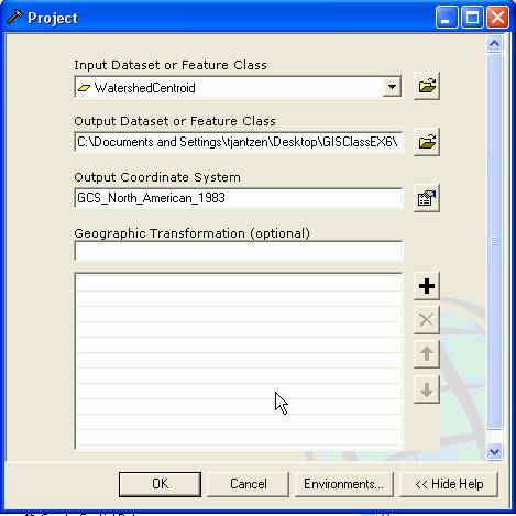
To use the Weather Downloader, the point feature class needs to be in Geographic Coordinates.� In the ArcToolbox browse to and click Data Management Tools > Projections and Transformations > Feature > Project.�
Use WatershedCentroid as the input feature class.� Keep the default name WatershedCentroid_Project.� Select the output projection to be North American Datum 1983.� Click OK.
You will also need to project the MonitoringPoint feature class.� The MonitoringPoint feature class will be used as the spatial reference for the USGS streamgage flow time series data.
Project the MonitoringPoint feature class to GCS_North_American_1983.� Title this new feature class MonitoringPoint_Project� Both of these feature classes are loaded into the ArcMap document and stored in the SanMarcos_ArcHydro geodatabase.
Using Weather
Downloader
We are now ready to download historical precipitation data for the centroid of each of our watersheds.� Install this tool by clicking on the Setup Icon that is shown below, and follow the instructions given.

�
In ArcMap select Tools/Customize, Add from File and choose C:\Program Files\CUAHSI\Weather Downloader and within that folder, WeatherDownloader.tlb and drag the WeatherDownloader button onto your ArcMap toolbar.
For further information on what to do once you have the tool installed , see
http://www.crwr.utexas.edu/gis/gishydro06/GISandHIS/Webservice_Ingestion_2006.htm
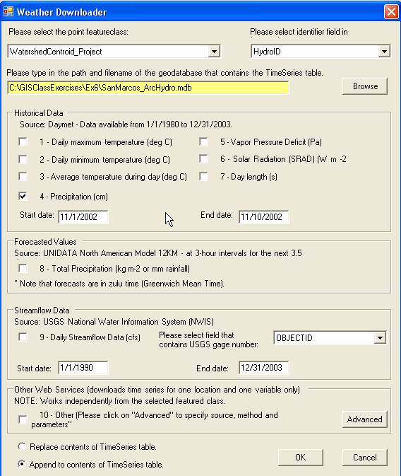
Click on the Weather
Downloader tool icon that you added during the installation of this
tool.� Use the WatershedCentroid_Project feature class as the dataset for which to
gather weather data.� Select HydroID as the identifier.� This will allow us to relate the downloaded
data to the watershed centroid, the watershed itself, and the watershed
outlet.� Browse to the location of the
SanMarcos_ArcHydro geodatabase for the location of the TimeSeries table.�� Note: you will have to do this manually, as
the default points somewhere else.� Check
the
As Weather Downloader gathers time series information, the points on the map will be highlighted. Be patient, as this process may take a few minutes.
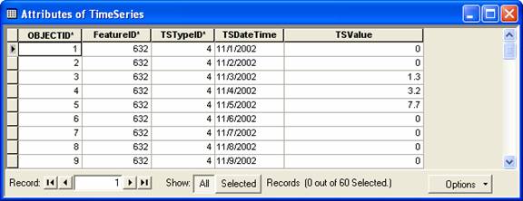
Once the Weather Downloader is complete, Open the TimeSeries table and look at its contents.� You should notice a series of historical precipitation data with TSDateTime values in the near future.�
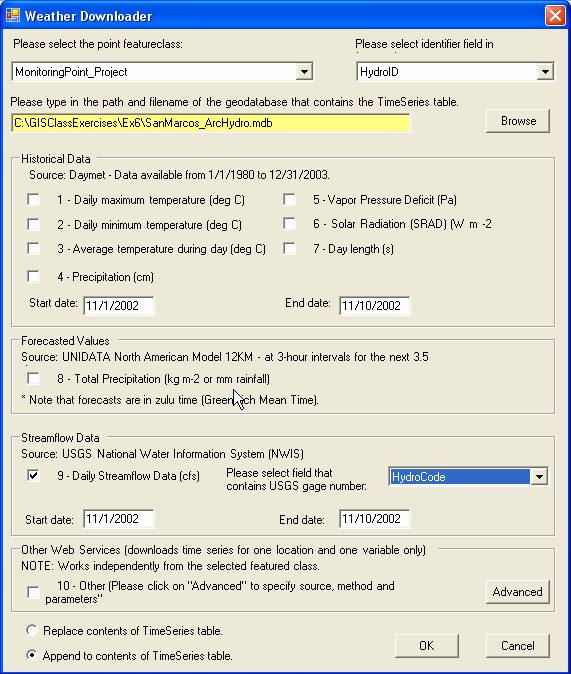
Repeat the Weather
Downloader process using MonitoringPoint_Project
as the source point featureclass.� We
will use the monitoring points (where are USGS gage sites) to download USGS
NWIS streamflow data for the same dates as we retrieved precipitation
data.� The identifier field should still
be HydroID, the location of the
TimeSeries table the same.� However, this
time, instead of checking the Precipitation box, check the 9- Daily Streamflow Data (cfs).�
To make this work correctly we need to identify the field in the
MonitoringPoint_Project featureclass that references the USGS Streamgage
number.� For this example, use HydroCode.� Select the same date range used for
precipitation.� Lastly, make sure that Append to contents of TimeSeries table is
still selected.� Otherwise, you may lose
the precipitation data you just downloaded.�
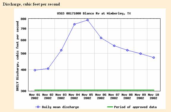
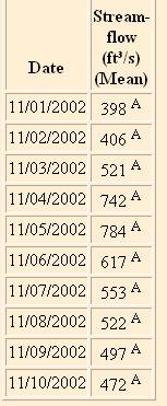
Lets check to make sure that we got the right data.�� Here are the downloaded streamflow values
for the MonitoringPoint at the
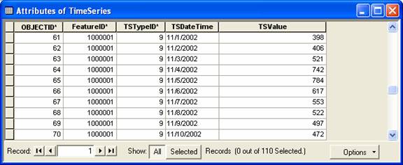
And here are the same data directly graphed from the USGS Water web site.�� A visual check suggests that these data are consistent.�� What has happened is that you have used CUAHSI web services to automatically download USGS data without using the USGS web site itself.� Ok, go CUAHSI!!� As a check, I downloaded the actual data as a table and everything looks swell!
Good job!� You have successfully used Weather Downloader to retrieve precipitation and streamflow data from web services for a historical storm event.
Viewing Temporal Data in
ArcGIS
Another useful task within ArcMap for utilizing ArcHydro is to simply visualize the spatial and temporal patterns of hydrologic phenomena (like rainfall or streamflow).� To do this, ESRI developed an extension for ArcMap called the Tracking Analyst.� If you don�t have tracking analyst, just stop the exercise here and skip the last part.
The Tracking Analyst is flexible in the format of data required and the options for symbolizing and rendering the spatial features according to the magnitude of their time series value for a given time-stamp.� The required information is a shape, a date, and a value (i.e. where, when, and what) that can be stored in one feature class or one feature class and one associated table.� This flexibility allows the Tracking Analyst to display features that move and/or change shape through time in addition to features that have time-indexed attribute values.� Below is a list of possible scenarios for features changing through space and over time:
- Stationary features with dynamic attribute (e.g. a stream flow gage)
- Stationary features with dynamic shape (e.g. an inundated river)
- Moving features with dynamic attribute (e.g. particle tracing in the subsurface)
- Moving features with dynamic shape (e.g. a hurricane)
Let�s get started with using Tracking Analyst ���
For this section of the exercise, we will visualize the
historical precipitation and streamflow for the
If the Tracking Analyst toolbar is not present on the ArcMap user interface, click View�Toolbars, and then select Tracking Analyst.� This displays the Tracking Analyst toolbar (shown below).�
Check to make sure the Tracking Analyst extension is selected (if not, the buttons on the Tracking Analyst will be disabled).� Click Tools�Extensions.� Click on the box next the �Tracking Analyst� if it is not already checked.
We will now create a Temporal Layer using the
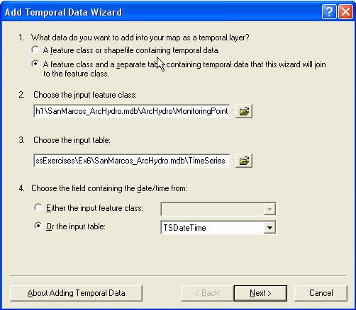
MonitoringPoint feature class and the TimeSeries table.� Click the ![]() �button on the Tracking Analyst toolbar.� Select the second option for the first
question (What data do you want to add into your map as a temporal layer),
browse to the input feature class (MonitoringPoint)
and then to the input table (TimeSeries).� Remember, the MonitoringPoint class
represents streamflow.� Finally, select TSDateTime from the input table as the
date/time field.� The form should look
like what�s pictured below.� Click Next.
�button on the Tracking Analyst toolbar.� Select the second option for the first
question (What data do you want to add into your map as a temporal layer),
browse to the input feature class (MonitoringPoint)
and then to the input table (TimeSeries).� Remember, the MonitoringPoint class
represents streamflow.� Finally, select TSDateTime from the input table as the
date/time field.� The form should look
like what�s pictured below.� Click Next.
On the next page, choose HydroID as the join field in the input feature class and FeatureID as the join field in the input table.� This will provide the link between features in the feature class and their associated time series records. Click Finish.� It should only take a second for ArcMap to generate the temporal layer named TimeSeries & MonitoringPoint.� Notice that this new layer is simply the MonitoringPoint features joined to TimeSeries time series table.� Open up the layer�s attribute table to take a look.
If you open the attribute table for the new temporal layer TimeSeries & MonitoringPoint,
you�ll see a table with 50 features, one representing each time series record
for each feature.� We�ll now symbolize
this layer to show the storms movement over the
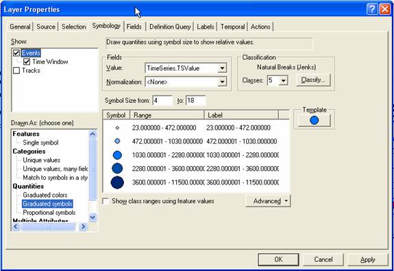
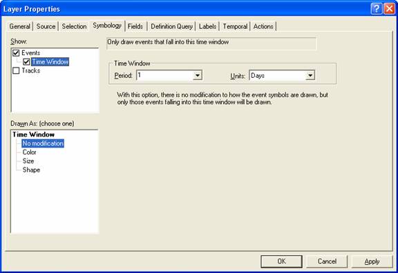
Now let�s symbolize the data.� Select the Symbology tab in the Layer Properties form.�
You�ll notice that the symbology tab for a temporal layer is somewhat different than one for a normal spatial layer.� In the top left corner in the Show box there are three options.� The Events option controls how the features are symbolized for each time step.� The Time Window option allows you to change the event symbology as time progresses.� The Tracks option can be used to connect features as they move through time (i.e. to show the path of an airplane as it moves).��
To symbolize the
Events:
Make sure the Events option is highlighted in the Show box.� In the Drawn As box, select Graduated symbols under the Quantities heading.�� For the Fields value, select TimeSeries.TSValue as the value (see figure below).�
Click the Classify button and chose to classify the values into 5 Quantiles.�
Color the symbols appropriately (I used light blue for low flow and dark blue for highest category of flow).
To set a Time Window:
In the Show box of the Symbology tab, check the box next to Time Window.� With Time Window highlighted, choose to limit the display of data to a one day time window.
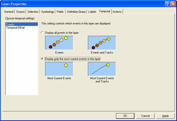
Finally, on the Temporal tab, select to show only the most current events.
Close the Layer Properties form.
You have now symbolized the temporal layer for rainfall and are ready to animate the rainfall over time.�
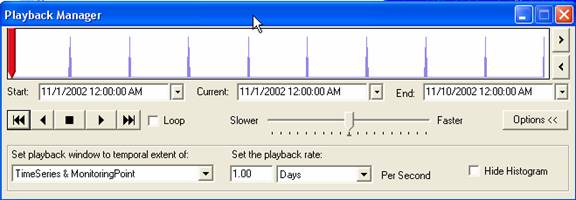
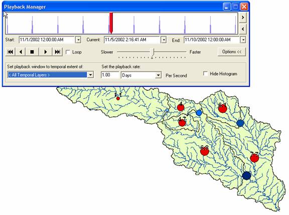
Press the ![]() �button on the Tracking Analyst toolbar.� This will launch the Playback Manager (shown
below).� Click Options and set the playback rate to 1 day.� You can press the play button to start the
animation, or just move the red bar to the right.� Try both.�
�button on the Tracking Analyst toolbar.� This will launch the Playback Manager (shown
below).� Click Options and set the playback rate to 1 day.� You can press the play button to start the
animation, or just move the red bar to the right.� Try both.�
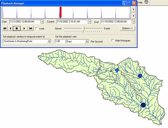
We can see that there was a large storm event during this
period with peak flow of over 11000 cfs averaged over a day.� To see the rain event that created this
streamflow, we�ll follow the same procedure outlined above to add a second
temporal layer for the rainfall gages in the
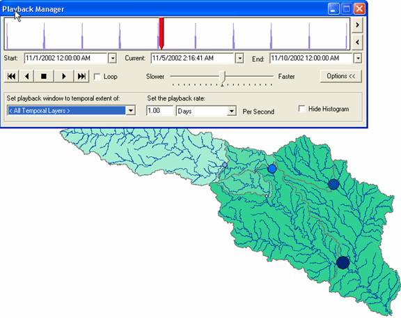
Create a second temporal layer following the same procedure.� This time, use the WatershedCentroid_Project. �When you�re done, you should be able to view the rainfall event and the resulting increase in stream flow.��
Alternatively, you may want to represent rainfall as a color for each watershed.� Remember that the rainfall data was collected for the centroid of the watershed.� Because the WatershedCentroid kept the same HydroID as Watershed, you can use Watershed as the feature class in the Temporal Data Wizard.� Then, instead of using graduated symbols, you could use graduated colors.�
Tracking Analyst can also be used to make a movie.� The movie can then be put into PowerPoint or on the web and act as a power visualization tool.
On the Tracking Analyst toolbar, press Tracking Analyst �
Animation Tool.� Keep the
While having the rainfall data geospatially reference by the Hydrologic Response Units (or the NEXRAD cells) is useful, potentially more useful is having the data geospatially referenced by the watersheds.� This is a first step in using the rainfall to estimate streamflow.� We�ll do this another time!
To be turned in:� Find the volume of rainfall (m3) that fell
over the watershed of the
Summary of items to
be turned in:
Items to be Turned In:
(1)�� A screen capture showing the results of an
Identify query for the Watershed, HydroJunction and Monitoring Point for the
(2)� Do
a trace from the most upstream junction in the network and �trace downstream�
to the outlet.�� What is the total length
(km) of the flow path thus identified? How many HydroJunctions are
selected?�� What stream gages measure
flow along this path (give the stream gage names and USGS ID values).�� What is the total area of the watersheds
that this flow path traverses?
(3)������� What
is the drainage area of DEM watershed draining to the gage on the
(4)������� A map of the watersheds, symbolized by the quantity of the Average AWC with the value for AvgAWC displayed on the map.��� Also include the Flowlines on this map.�
(5)������� Find
the volume of rainfall (m3) that fell over the watershed of the