Watershed and Stream Network Delineation
GIS in Water Resources
Fall 2005
Prepared by Venkatesh Merwade, David Maidment and Oscar
Robayo
Center
for Research in Water Resources
Contents
Computer and
Data Requirements
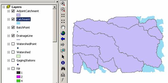
Open ArcMap and load Arc Hydro tools
8. Catchment
Polygon Processing
10. Adjoint
Catchment Processing
12. Drainage
Density Evaluation
1. Batch
Watershed Delineation
2. Interactive
Point Delineation
3. Batch
Subwatershed Delineation
Appendix.
Procedures for correcting problems with vector processing due to X/Y
domain problems.
Purpose
The purpose of this
exercise is to illustrate, step-by-step, how to use the major functionality
available in the Arc Hydro tools for Raster Analysis. In this exercise, the user will
perform drainage analysis on a terrain model for the
Computer and Data Requirements
To
carry out this exercise, you need to have a computer, which runs the ArcInfo version of ArcGIS. The data
are provided in the accompanying zip file, Ex52005.zip available at http://www.engineering.usu.edu/dtarb/giswr/Ex52005.zip. The
data files used in the exercise consist of DEM grid for the
Data description:
The
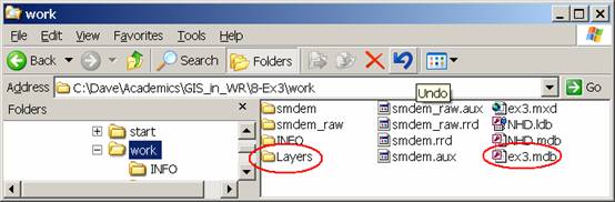
contents of Ex52005.zip when unzipped are illustrated below:
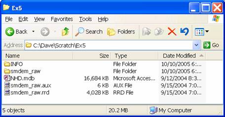
The
geodatabase NHD.mdb contains data from the National Hydrography dataset. Inside NHD.mdb, we are interested in
NHDFlowline and USGSGage feature classes stored in the Hydrography feature
dataset and Subbasin feature class contained in the HydrologicUnits feature
dataset. The USGSGage feature class is
the same USGSgage feature class used in an earlier exercise. The folder smdem_raw and associated files
smdem_raw.aux, smdem_raw.rrd and files in the INFO folder contains the digital
elevation model for this region obtained from the National Elevation
dataset. (Remember that in ArcGIS single
datasets are often stored in multiple files on the computer and these files
should be manipulated using ArcCatalog.
If you move the files using the Windows Explorer you may omit one of
them and corrupt the data. Following is
the ArcCatalog depiction of the data files provided

Getting Started
Open ArcMap and load Arc Hydro tools
Make sure the Arc Hydro tools are installed on the system. This should already have been installed in the LRC lab at UT. It has not been installed (yet) in the lab at USU but only takes a few minutes to install. The ArcHydro installation file may be obtained from http://www.crwr.utexas.edu/gis/gishydro05/ArcHydro/ArcHydroTools.htm. Click on Download Arc Hydro Tools (.exe), save and run the executable file you receive.
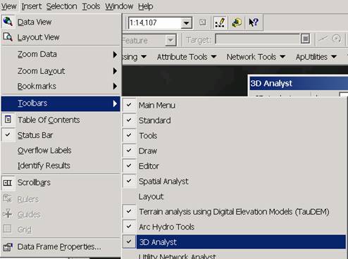
Open ArcMap. Create a new empty map, and save it as Ex5.mxd (or any other name). Right click on the menu bar to pop up the context menu showing available tools as shown below.
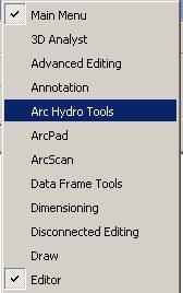
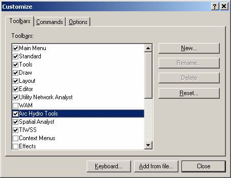
Check the Arc Hydro Tools menu. If the Arc Hydro Tools menu does not appear in the list, click on “Customize” (Scroll down the list to see “Customize”). In the Customize dialog that appears, check the Arc Hydro Tools box.
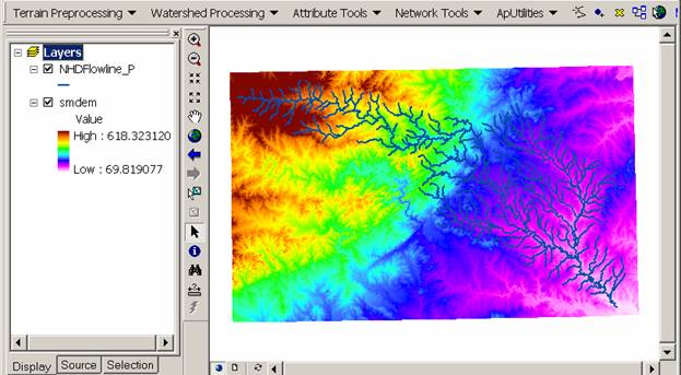
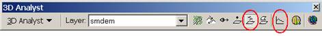
You should now see the Arc Hydro tools added to ArcMap as shown below. You can leave it floating or you may dock it in ArcMap.
![]()
Note
It is not necessary to load the Spatial Analyst, Utility Network Analyst, or Editor tools because Arc Hydro Tools will automatically use their functionality on as needed basis. These toolbars need to be loaded though if you want to use any general functionality that they provide (such as general editing functionality or network tracing).
However, the Spatial Analyst Extension needs to be activated, by clicking Tools>Extensions…, and checking the box next to Spatial Analyst.
Dataset
Setup
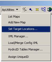
The existing NHD data to be used in this exercise are stored in a geodatabase and loaded in the map. All vector data created with the Arc Hydro tools will be stored in a new geodatabase that has the same name as the stored project or ArcMap document (unless pointed to an existing geodatabase) and in the same directory where the project has been saved (your folder for Ex5). By default, the new raster data are stored in a subdirectory with the same name as the dataset or Data Frame in the ArcMap document (called Layers by default and under the directory where the project is stored). The location of the vector, raster, and time series data can be explicitly specified using the function ApUtilities>Set Target Locations.
You can leave the default settings if they are pointing to the same directory where the ArcMap document is saved.
Load the data to ArcMap
Click on the ![]() icon to add the raster
data. In the dialog box, navigate to the location of the data; select the
raster file smdem_raw containing the DEM for
icon to add the raster
data. In the dialog box, navigate to the location of the data; select the
raster file smdem_raw containing the DEM for ![]() in ArcMap to display ArcToolbox. In
ArcToolbox, select Data Management ToolsàProjections and
TransformationsàRasteràProject
Raster as shown below:
in ArcMap to display ArcToolbox. In
ArcToolbox, select Data Management ToolsàProjections and
TransformationsàRasteràProject
Raster as shown below:

Double click on “Project Raster” to get the following form:
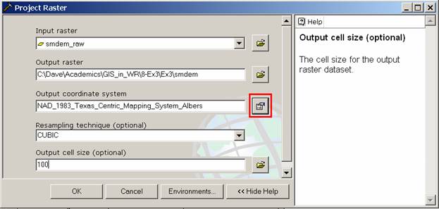
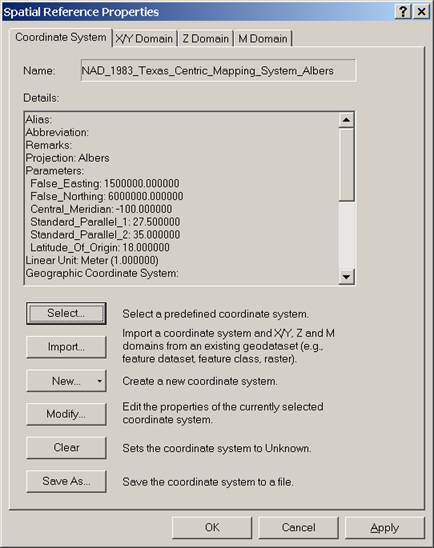
The input raster is smdem_raw already added to ArcMap, name the output raster as smdem, choose the output coordinate system by clicking at the button next to the input text-box to get the following form:
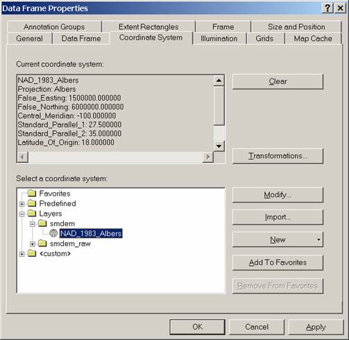
Then click on ![]() in the table of contents, click on PropertiesàCoordinate
System and assign the coordinate system of smdem to the map document as shown
below:
in the table of contents, click on PropertiesàCoordinate
System and assign the coordinate system of smdem to the map document as shown
below:
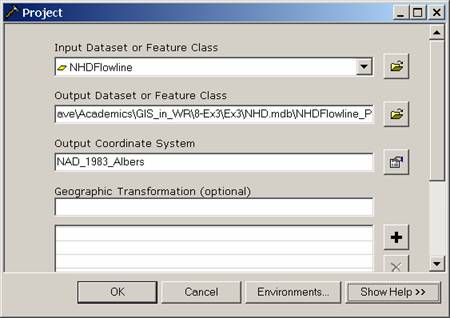
After defining the coordinate system for the map document, add NHDFlowline feature class from the Hydrography feature dataset within NHD.mdb. The NHDFlowline feature class has geographic coordinate system. Project the NHD Flowline feature class by using the ArcTool box. Click on Data Management ToolsàProjections and TransformationsàFeatureàProject. The input feature class is NHDFlowline. Save the output feature class as NHDFlowline_P within the NHD.mdb geodatabase, and import a coordinate system from smdem to project the flowlines to the same coordinate system as smdem (NAD_1983_Albers).
Remove the layers Smdem_raw and NHDFlowline from the ArcMap document. From now on we will work with projected data and do not want to inadvertently use the raw data that does not have the correct projection. Save and close the ArcMap document. You are now ready for terrain analysis! (Closing and reopening ArcMap has the effect of making the system "forget" some of the internal information involved with projections that confounds the ArcHydro processing later.)
Exploring the DEM
The spatial information about the DEM can be found by right clicking on the smdem layer, then clicking on PropertiesàSource. Similarly, the symbology of the DEM can be changed by right clicking on the layer, PropertiesàSymbology.

To be turned in: Cell size, Number of rows and columns of smdem, maximum and minimum elevation values in smdem.
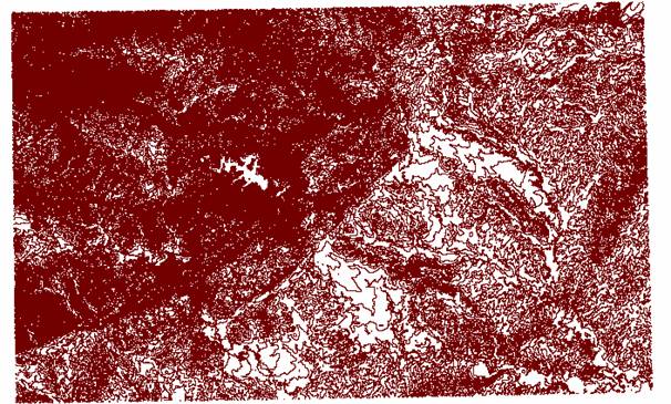
To explore the highest elevation areas in your DEM Select Spatial
Analyst/Raster Calculator. If you
don’t see the Spatial Analyst toolbar, go to View/Toolbars and click on
Spatial Analyst. Double click on the
layer smdem with the DEM for

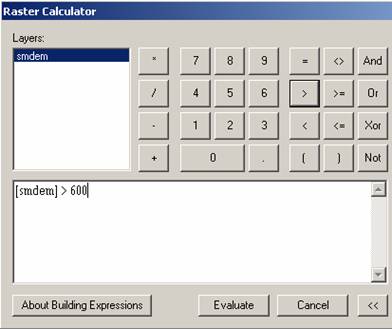
A new layer called calculation appears on your map. The majority of the map (brown color in the figure below) has a 0 value representing false (values below the threshold), and the red region has a value of 1 representing true (elevations higher than 550 meters).
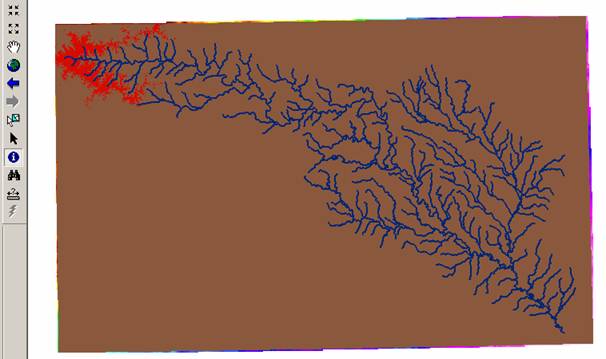
Zoom in to the region of highest elevations (red region) and
do some sampling on the smdem grid using the identify ![]() tool to select a point close to the maximum
elevation. In a layout mark your point of maximum elevation and label it with
the elevation value for that pixel.
tool to select a point close to the maximum
elevation. In a layout mark your point of maximum elevation and label it with
the elevation value for that pixel.
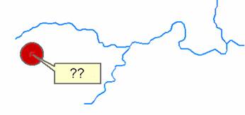
You can place the dot using the Draw toolbar. It seems that when you zoom out the dot does not show up in zoomed out view. If that is the case, just show the zoomed-in view, as above.
Contours
Contours are a useful way to visualize topography. This can be done by using the spatial analyst extension through the following steps:
Select Spatial Analyst > Surface Analysis
> Contour…
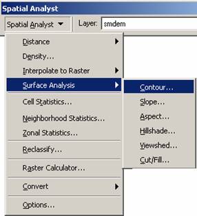
Select the Input surface as smdem, leave the default parameters, and browse to your output folder. Name output features as contour.shp. If you find that you don’t have contours over your whole extent, it is because one of your Calculation grids has been chosen by default as the Input surface. Make sure smdem is provided as the input surface.

A layer is generated with the topographic contours for
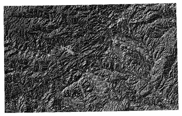
Another option to provide a nice visualization of topography is Hillshading.
Select Spatial Analyst > Surface Analysis > Hillshade… and set the factor Z to a higher value to get a dramatic effect and leave the other parameters at their defaults (the following hillshade is produced with a Z factor of 100). Click OK. You should see an illuminated hillshaded view of the topography.
To be turned in: A
layout with a depiction of topography either with contours or hillshade in nice
colors. Include the streams from NHD (NHDFlowline). Mark your point of highest
elevation and indicate its elevation.
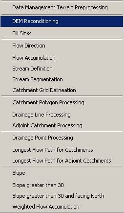
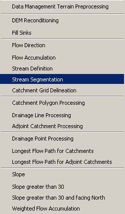
Terrain Preprocessing
Terrain
Preprocessing uses DEM to identify the surface drainage pattern. Once preprocessed, the DEM and its
derivatives can be used for efficient watershed delineation and stream network
generation.
All the steps in the Terrain Preprocessing menu should be performed in sequential order, from top to bottom. All of the preprocessing must be completed before Watershed Processing functions can be used. DEM reconditioning and filling sinks might not be required depending on the quality of the initial DEM. DEM reconditioning involves modifying the elevation data to be more consistent with the input vector stream network (NHD). This implies an assumption that the stream network data are more reliable than the DEM data, so you need to use knowledge of the accuracy and reliability of the data sources when deciding whether to do DEM reconditioning. By doing the DEM reconditioning you can increase the degree of agreement between stream networks delineated from the DEM and the input vector stream networks.
In general you should be aware that some of the terrain
processes may take a long time to finish. Processes like DEM Reconditioning, Filling
Sinks and Flow accumulation can take 10 to 15 minutes each for a grid with around
4000 x 4000 rows and columns. In this
exercise the grid resolution has been degraded to 100 m to expedite the
processing.
1. DEM Reconditioning
This function modifies a DEM by imposing linear features
onto it (burning/fencing). It is an implementation of the AGREE method
developed Center for Research in Water Resources at the
The function needs as input a raw dem and a linear feature class (like the river network) that both have to be present in the map document.
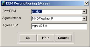
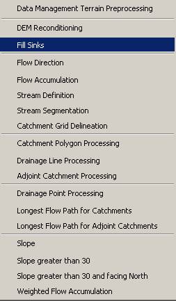
Select Terrain Preprocessing | DEM Reconditioning.
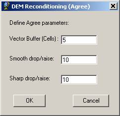
Select the appropriate Raw DEM (smdem) and AGREE stream feature (NHDFlowline_P). Click OK to accept the default Agree parameters. The output is a reconditioned Agree DEM (default name AgreeDEM).
This process takes about 2 to 3 minutes! Examine the folder where you are working you will notice that a folder named Layers has been created. This is where ArcHydro outputs its grid results. A personal geodatabase with the same name as your ArcMap document has also been created. This is where ArcHydro outputs its vector feature class data.
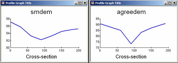
If you are curious you can examine what AGREE has done to the DEM. First examine AgreeDEM properties®Source. Check that the cellsize and number of rows and columns are the same as the original DEM. If these are changed then Agree has performed some sort of interpolation, which seems to occur if projections have been changed and can be avoided by closing and re-opening the ArcMap document. Next use 3D analyst to examine profiles across streams. Check that 3D Analyst is checked under Tools®Extensions. Then Activate 3D Analyst on View®Toolbars
Use the Interpolate Line and Create Profile Graph tools to examine a profile cross section across a stream.
2. Fill Sinks
This function fills the sinks in a grid. If cells with higher elevation surround a cell, the water is trapped in that cell and cannot flow. The Fill Sinks function modifies the elevation value to eliminate these problems.
Select Terrain Preprocessing | Fill Sinks.
Confirm that the input for DEM is “AgreeDEM” (or your original DEM if Reconditioning was not implemented). The output is the Hydro DEM layer, named by default “Fil”. This default name can be overwritten.
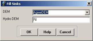
Press OK. Upon successful completion of the process, the “Fil” layer is added to the map. This process takes a few minutes.
3. Flow Direction
This function computes the flow direction for a given grid. The values in the cells of the flow direction grid indicate the direction of the steepest descent from that cell.
Select Terrain Preprocessing | Flow Direction.
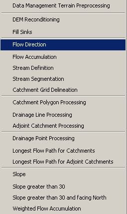
Confirm that the input for Hydro DEM is “Fil”. The output is the Flow Direction Grid, named by default “Fdr”. This default name can be overwritten.
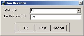
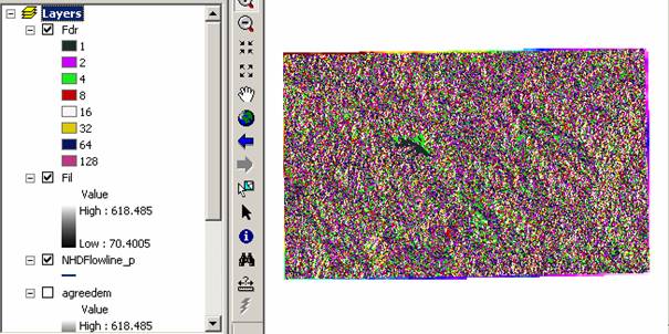
Press OK. Upon successful completion of the process, the flow direction grid “Fdr” is added to the map.
4. Flow Accumulation
This function computes the flow accumulation grid that contains the accumulated number of cells upstream of a cell, for each cell in the input grid.
Select Terrain Preprocessing | Flow Accumulation.
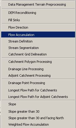
Confirm that the input of the Flow Direction Grid is “Fdr”. The output is the Flow Accumulation Grid having a default name of “Fac” that can be overwritten.
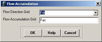
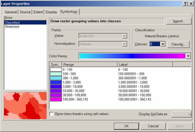
Press OK. Upon successful completion of the process, the flow accumulation grid “Fac” is added to the map. This process may take several minutes for a large grid! Adjust the symbology of the Flow Accumulation layer "Fac" to a multiplicatively increasing scale to illustrate the increase of flow accumulation as one descends into the grid flow network.
After applying this layer symbology you may right click on the "Fac" layer and Save As Layer File
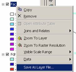
The saved Layer File may be imported to retrieve the symbology definition and apply it to other data.
Add the
The value obtained represents the drainage area in number of 100 x 100 m grid cells. Calculate the drainage area in km2.
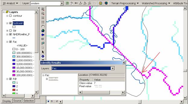
Also examine the southern rim of the basin where there is a NHD stream crossing the NHD subbasin boundary.
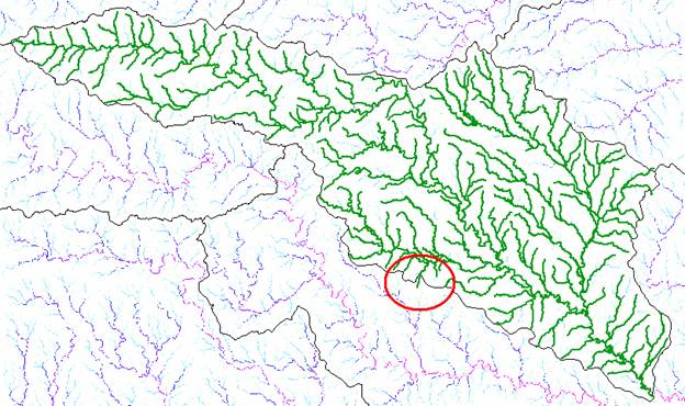
Zoom in on this location and use identify to determine the value of "fac" at the point where this small stream "enters" the delineated HUC. Determine the corresponding area in km2. If we assume that the DEM (from NED) and NHD flowline data is higher quality than the NHD subbasin boundary this indicates an omission of area due to inaccurate delineation of the subbasin boundary.
To be turned in: Report the drainage area of the San Marcos basin in both number of 100 m grid cells and km2 as estimated by flow accumulation. Report the omitted drainage area assumed due to imprecise delineation at the location indicated on the southern edge, in both number of 100 m grid cells and km2.
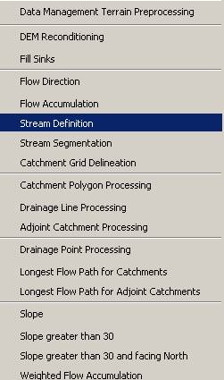
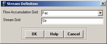
5. Stream Definition
This function computes a stream grid which contains a value of "1" for all the cells in the input flow accumulation grid that have a value greater than the given threshold. All other cells in the Stream Grid contain no data.
Select Terrain Preprocessing | Stream Definition.
Confirm that the input for the Flow Accumulation Grid is “Fac”. The output is the Stream Grid. “Str” is its default name that can be overwritten.
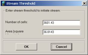
A default value is displayed for the river threshold. This value represents 1% of the maximum flow accumulation: a simple rule of thumb for stream determination threshold. The threshold drainage area to generate a stream is then 3601 x 100 x 100 / 1000000 = 36 km2. However, any other value of threshold can be selected. For example, the USGS Elevation Derivatives for National Applications (EDNA http://edna.usgs.gov/) approach uses a threshold of 5000 30 x 30 m cells (an area of 4.5 km2) for catchment definition. A smaller threshold will result in a denser stream network and usually in a greater number of delineated catchments. Objective methods for the selection of the stream delineation threshold to derive the highest resolution network consistent with geomorphological river network properties have been developed and implemented in the TauDEM software (http://www.engineering.usu.edu/dtarb/taudem.)
Press OK. Upon successful completion of the
process, the stream grid “Str” is added to the map.

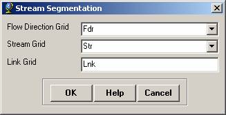
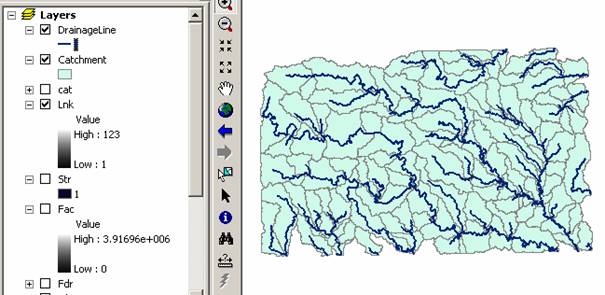
6. Stream Segmentation
This function creates a grid of stream segments that have a unique identification. Either a segment may be a head segment, or it may be defined as a segment between two segment junctions. All the cells in a particular segment have the same grid code that is specific to that segment.
Select Terrain Preprocessing | Stream Segmentation.
Confirm that “Fdr” and “Str” are the inputs for the Flow Direction Grid and the Stream Grid respectively. The output is the Link Grid, with the default name “Lnk” that can be overwritten.
Press OK. Upon successful completion of the process, the link grid “Lnk” is added to the map.
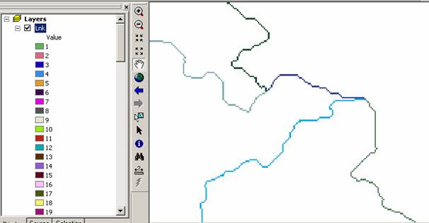
At this point, notice how each link has a separate value.
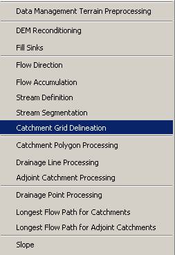
7. Catchment Grid Delineation
This function creates a grid in which each cell carries a value (grid code) indicating to which catchment the cell belongs. The value corresponds to the value carried by the stream segment that drains that area, defined in the stream segment link grid
Select Terrain Preprocessing | Catchment Grid Delineation.
Confirm that the input to the Flow Direction Grid and Link Grid are “Fdr” and “Lnk” respectively. The output is the Catchment Grid layer. “Cat” is its default name that can be overwritten by the user.
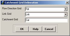
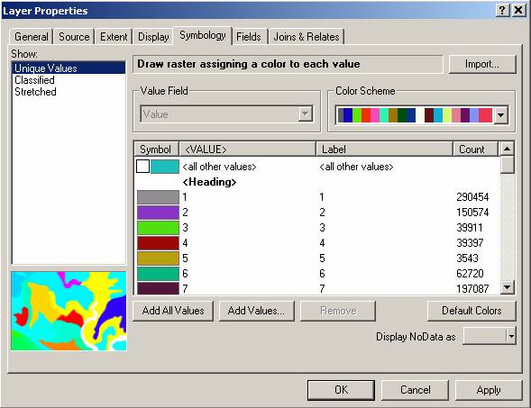
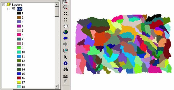
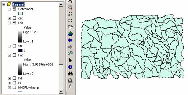
Press OK. Upon successful completion of the process, the Catchment grid “Cat” is added to the map. You can recolor the grid with unique values to get a nice display.
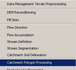
8. Catchment Polygon Processing
The three functions Catchment Polygon Processing, Drainage Line Processing and Adjoint Catchment Processing convert the raster data developed so far to vector format. The rasters created up to now have all been stored in a folder named "Layers". The vector data will be stored in a feature dataset also named "Layers" within the geodatabase associated with the map document. Unless otherwise specified under APUtilities®Set Target Locations the geodatabase inherits the name of the map document (Ex5.mdb in this case) and the folder and feature dataset inherit their names from the active data frame which by default is named "Layers".
Select Terrain Preprocessing | Catchment Polygon Processing.
This function converts a catchment grid into a catchment polygon feature.
Confirm that the input to the CatchmentGrid is “Cat”. The output is the Catchment polygon feature class, having the default name “Catchment” that can be overwritten.
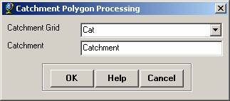
Press OK. Upon successful completion of the process, the polygon feature class “Catchment” is added to the map.
Open the attribute table of "Catchment". Notice that each catchment has a HydroID assigned that is the unique identifier of each catchment within ArcHydro. Each catchment also has Shape Length and Area attributes. These quantities are automatically computed when a feature class becomes part of a geodatabase.
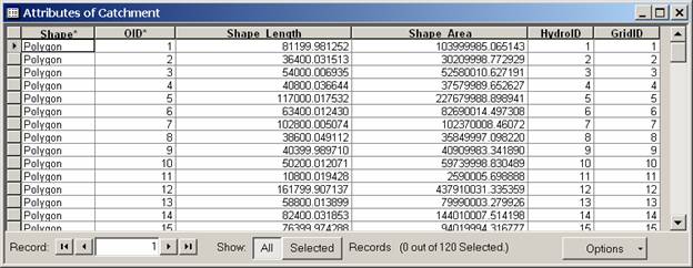
If any catchments are missing Length or Area this would be symptomatic of a problem with the X/Y domain of the feature dataset that ArcHydro created that occurred with earlier versions of Arc Hydro. If this problem occurs for you refer to the appendix for how to correct it.
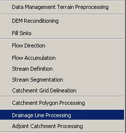
9. Drainage Line Processing
This function converts the input Stream Link grid into a Drainage Line feature class. Each line in the feature class carries the identifier of the catchment in which it resides.
Select Terrain Preprocessing | Drainage Line Processing.
Confirm that the input to Link Grid is “Lnk” and to Flow
Direction Grid “Fdr”. The output Drainage Line has the default name
“DrainageLine”, that can be overwritten.
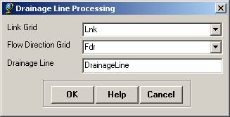
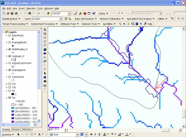
Press OK. Upon successful completion of the process, the linear
feature class “DrainageLine” is added to the map.
Compare the drainage lines delineated from the DEM procedure with the NHD flowlines.
To be turned in: A
layout with a comparison of the generated DrainageLine and the NHD river
network for
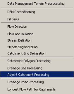
10. Adjoint Catchment Processing
This function generates the aggregated upstream catchments from the "Catchment" feature class. For each catchment that is not a head catchment, a polygon representing the whole upstream area draining to its inlet point is constructed and stored in a feature class that has an "Adjoint Catchment" tag. This feature class is used to speed up the point delineation process.
Select Terrain Preprocessing | Adjoint Catchment Processing.
Confirm that the inputs to Drainage Line and Catchment are respectively “DrainageLine” and “Catchment”. The output is Adjoint Catchment, with a default name “AdjointCatchment” that can be overwritten.
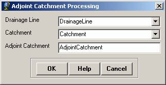
Press OK. Upon successful completion of the process, the polygon feature class “AdjointCatchment” is added to the map.
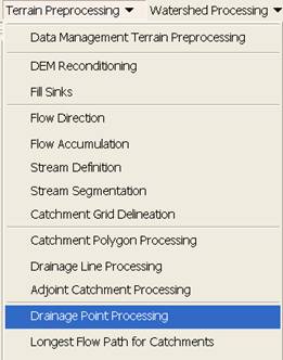
11. Drainage Point Processing
This function allows generating the drainage points associated to the catchments.
Select Terrain Preprocessing | Drainage Point
Processing.
Confirm that the inputs are as below. The output is Drainage Point, having the default name “DrainagePoint” that can be overwritten.
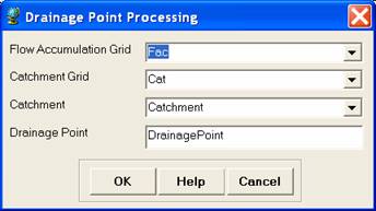
Press OK. Upon successful completion of the process, the point feature class “DrainagePoint” is added to the map.
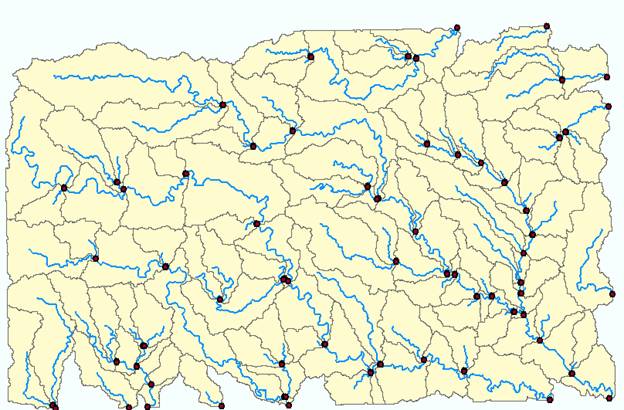
To turn in: How many DrainagePoints, DrainageLines and Catchments are there? What is the ID field in each feature class that associates the appropriate DrainagePoint with its DrainageLine and Catchment? Make a graphic showing how one associated DrainagePoint, DrainageLine and Catchment are related.
12. Drainage Density Evaluation
Now we will do some analysis to evaluate the drainage
density of the
The attribute table of the Subbasin feature class within the
HydrologicUnits feature dataset in the NHD geodatabase gives a shape area but
the units of this are decimal degrees because the spatial reference of this
feature class is geographic coordinates.
To evaluate the area of the

Designate the output feature class as one named "Subbasin" within the project geodatabase feature dataset "Layers".

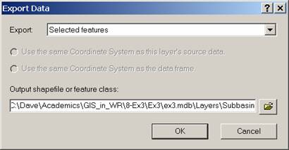
Click OK to add the exported data to the map. Open the attribute table of the feature class "Subbasin".
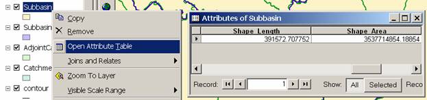
Notice that this has an attribute Shape Area that was created during the export of the feature class and is consistent with the spatial reference of the "Layers" feature dataset. This area is therefore in m2 and may be compared to the drainage area obtained from flow accumulation. Note this drainage area.
Next we'll calculate the length associated with the
DrainageLine feature class delineated from the DEM. This feature class includes streams outside
the
Select features from "DrainageLine" that intersect 'Subbasin" in the dialog below:
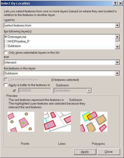
Click Apply and Close.
The DrainageLine features that intersect with the
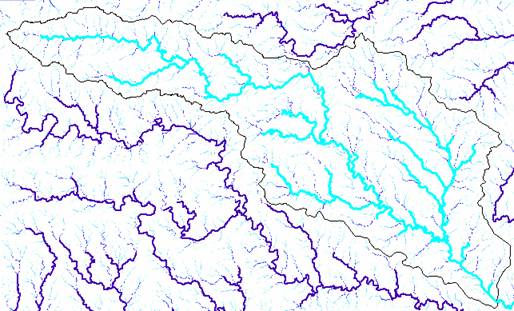
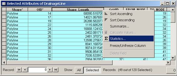
Open the attribute table associated with DrainageLine and Click Show "Selected"
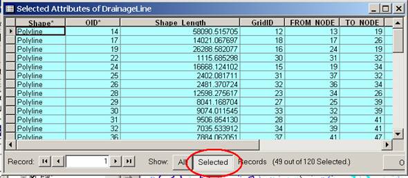
Right Click on Shape Length and select Statistics. Note the Sum in the statistics that are
displayed. This represents the length of
DrainageLine features that intersects with the
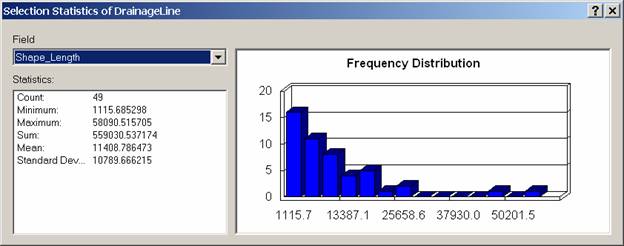
Open the attribute table of the projected NHDFlowline feature class and use Statistics on Shape Length to obtain the total length of streams from NHD.
To turn in: Report the drainage area of the
Watershed Processing
Arc Hydro also provides an extensive set of tools for delineating watersheds and subwatersheds. These tools rely on the datasets derived during terrain processing. This part of the exercise will expose you to some of the Watershed Processing functionality in Arc Hydro.
1. Batch Watershed Delineation
This function delineates the watershed upstream of each point in an input Batch Point feature class.
The Arc Hydro tools Batch Point Generation ![]() can be used to
interactively create the Batch Point feature class. We will use this to locate the outlet of the
watershed. Arrange your display so that
the san Marcos HUC 8 outline (subbasin), fac, DrainageLine and NHDFlowline_P
datasets are visible. Zoom in near the
outlet of the
can be used to
interactively create the Batch Point feature class. We will use this to locate the outlet of the
watershed. Arrange your display so that
the san Marcos HUC 8 outline (subbasin), fac, DrainageLine and NHDFlowline_P
datasets are visible. Zoom in near the
outlet of the ![]() in the Arc Hydro Tools
toolbar. Click on the outlet grid cell
where the
in the Arc Hydro Tools
toolbar. Click on the outlet grid cell
where the
Confirm that the name of the batch point feature class is “BatchPoint”. A point is then created at the location of mouse click, and the following form is displayed:
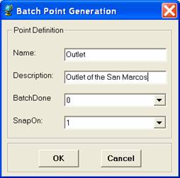
Fill in the fields Name and Description.
Both are string fields. The BatchDone and SnapOn options can be used to
turn on (select 1) or off (select 0) the batch processing and stream snapping
for that point. Select the options shown above. The input information is saved
in the attribute table of the BatchPoint feature class. Click OK.
You should see that a single point feature class has been created
comprising the outlet point where you clicked.
When snapping is turned on, if your point is sufficiently near to a drainage line (within around 5 grid cells) then the point will be snapped (i.e. moved) to a nearby drainage line before delineation of the upstream watershed, otherwise the local watershed draining to the point will be delineated. The following figure indicates the behavior you may expect from the delineation of watersheds upstream of input Batch Points.
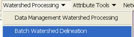
To perform a batch watershed delineation
Select Watershed Processing | Batch Watershed Delineation.
Confirm that “Fdr” is the input to Flow Direction Grid, “Str” to Stream Grid, “Catchment” to Catchment, “AdjointCatchment” to AdjointCatchment, and “BatchPoint” to “Batch Point”. For output, the Watershed Point is “WatershedPoint”, and Watershed is “Watershed”. “WatershedPoint” and “Watershed” are default names that can be overwritten.
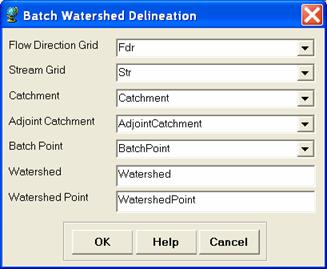
Press OK. The following message box appears on the screen, indicating that 1 point has been processed.
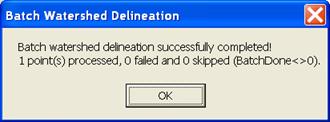
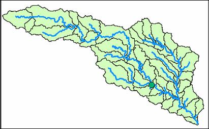
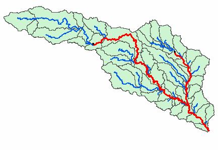
The delineated watersheds for the selected point should
correspond closely to the outline of the
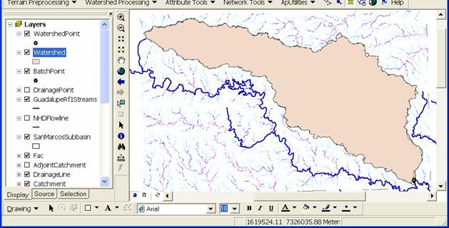
To be turned in: Make a layout showing the delineated watershed for your selected outlet. Report the Drainage Area of the watershed you delineated in km2.
Delineating Watersheds from USGS
gaging stations:
Add the USGSgage feature
class from the Hydrography feature dataset within the NHD.mdb geodatabase. Click OK if you receive the warning about the
data being in a different projection.
This is actually a "good" warning. It means that ArcGIS knows about the
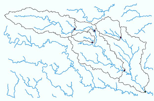
difference in projections and will project on the fly. These are the locations of the USGS gages
within the
To use these gages as watershed outlets these locations need to be appended to the Batchpoint feature class.
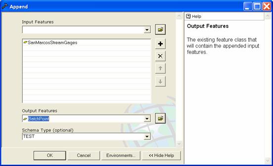
Open the Append tool.

Set the input to SanMarcosStreamGages and Set the Output to BatchPoint. Click OK.
Open the BatchPoint Attribute table.
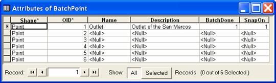
Notice that the 5 points from the SanMarcosStreamGages feature class have been appended to the outlet already there. To use these within Watershed Delineation we need to set the BatchDone and SnapOn fields. Select the 5 new records in the attribute table to perform calculations on a selection. Right click on the BatchDone header and select Calculate Values.
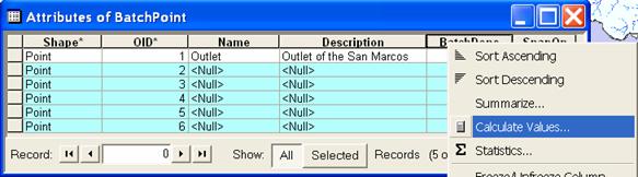
Click Yes to the field calculator warning about the calculations not being reversible.
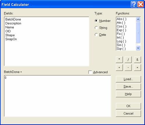
Enter 0 in the BatchDone= field and click OK.
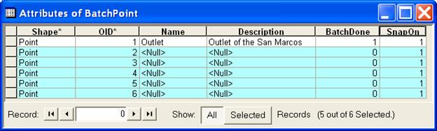
Notice that all the BatchDone values are set to 0. Similarly set SnapOn equal to 1. The result should be as follows.
Close the attribute table and repeat the Watershed ProcessingàBatch Watershed Delineation function. The Watersheds draining to each stream gage should be delineated.
If you zoom in close to a gage location you will see that a WatershedPoint has been created on the stream very near to the USGS gage. This is the effect of snapping and accommodates the fact that USGS gage locations are not precisely aligned with the streams we delineated.
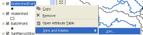
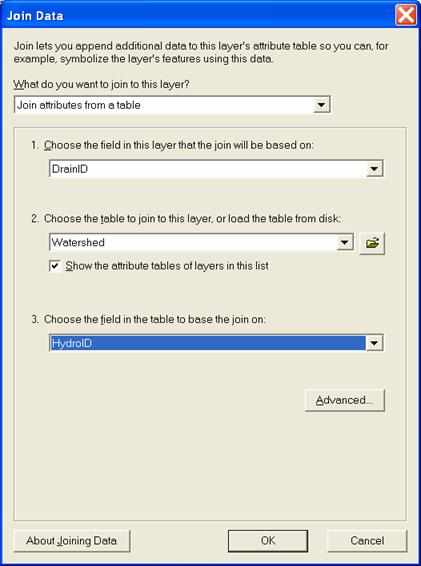
The attributes, such as names and USGS Station Number are not yet associated with the delineated watershed pointss. To remedy this we will use a Join based on spatial location to the USGSgage feature class. Right click on WatershedPoint/Joins and relates/Join
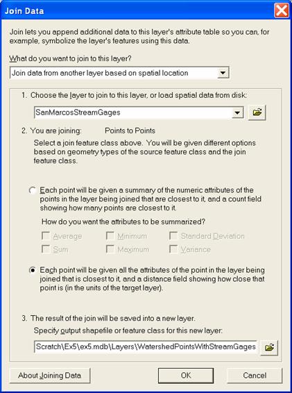
In the Join Data dialog specify Join data from another layer based on spatial location. Specify the layer to join to this layer as SanMarcosStreamGages. Under 2 specify each point given all the attributes in the layer closest to it. Specify the output feature class as Ex5.mdb\Layers\WatershedPointsWithStreamGages.
The attribute table of WatershedPointsWithStreamGages now includes all the USGS Stream Gaging station data. We would now like to associated watershed attributes, such as drainage area from the Watershed feature class with these stream gages.
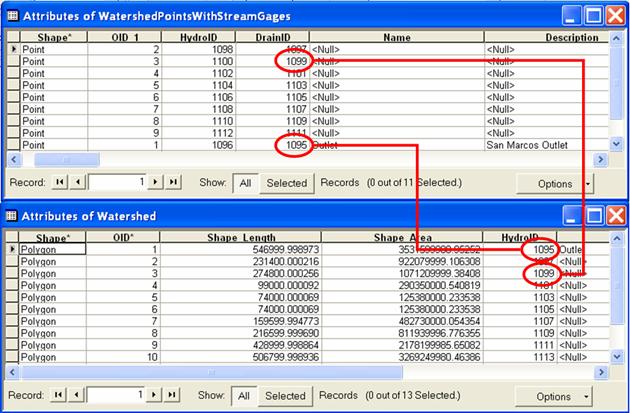
Open the attribute table for the "Watershed" feature class. Notice that it contains a field "HydroID". This is a unique identifier associated with each Watershed. The attribute table of "WatershedPointsWithStreamGages" contains fields "HydroID" and "DrainID". HydroID is again unique (i.e. different from the HydroID of Watersheds and all other objects) because Points are separate objects from Watersheds. The DrainID field gives the relationship between these tables with "DrainID" in WatershedPoints giving the HydroID of the corresponding Watershed. We can therefore join the Watersheds attribute table onto the WatershedPoints table to associate watershed attributes with their outlet points.
Right click on WatershedPointsWithStreamGages and select Joins and Relates/Join. Select to Join attributes from a table and select "DrainID" as the join field in this layer (WatershedPointsWithStreamGages). Select the "Watershed" table and HydroID field to join. Click OK.
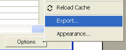
Click No to create index (indices are only really beneficial for large tables). Open the table attribute table for WatershedPointsWithStreamGages which now has watershed attributes joined to it. Note that this single (rather broad) table displays the watershed attributes adjacent to details of each stream gage. The most important attribute is Watershed area, because this is a quantity very important in properly interpreting streamflow. Click Options®Export to export the data into a DBF table.
Open the DBF table that you obtain in Excel and use Excel to tidy it up and produce a presentation quality table that gives for each outlet point the following information:
Name, USGS gage number, Watershed point HydroID, Watershed HydroID, Drainage area from ArcGIS (converted km2).
To be turned in: Make a layout showing the delineated watershed for each USGS Gauging Station. Label each watershed outlet with its contributing Drainage Area obtained from the Watershed Feature class. Prepare a table using Excel giving Name, USGS gage number, Watershed point HydroID, Watershed HydroID, Drainage area from ArcGIS (converted km2).
2. Interactive Point Delineation
An alternative to delineate watersheds when you do not want
to use the batch mode (process a group of points simultaneously) to generate
the watershed for a single point of interest is the Point Delineation tool ![]() .
.
Click on the Point Delineation icon ![]() in the ArcHydro
toolbar to activate the tool. Zoom in to the network and click the mouse (along
the drainage line) to create your point of interest.
in the ArcHydro
toolbar to activate the tool. Zoom in to the network and click the mouse (along
the drainage line) to create your point of interest.
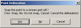
Click “Yes” if the following message is displayed.
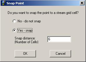
Press OK to snap the point to a stream grid cell (this form
will not be presented if the point is already on the stream).
After the delineation is complete, fill in the name and comment as shown below in the form.
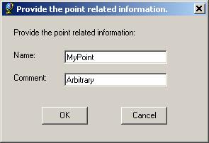
After all the information is fed, a watershed will be added to the “Watershed” feature class, and the point you created is added to the “WatershedPoint” feature class.
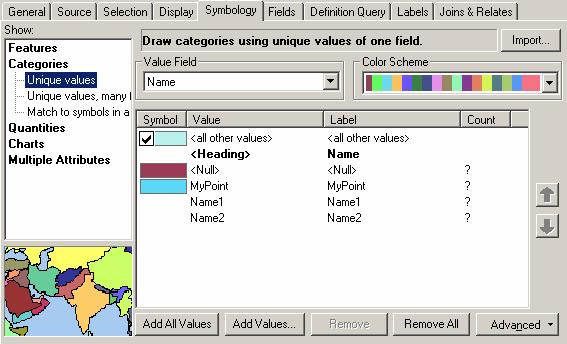
To show only the
new watershed from the watershed feature class, use symbologyàUnique Valueà use “Name” for the value field, and use
Hollow symbols for other fields with “0” value for border width.
The delineated watershed for the selected point is shown below.
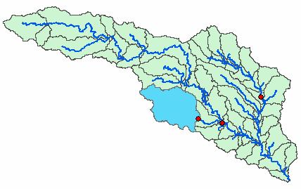
To be turned in: Make a layout showing the delineated watershed for your selected point including the DrainageLine and the Catchments
3. Batch Subwatershed Delineation
This function delineates subwatersheds for all the points in a selected Point Feature Class.
Input to the batch subwatershed delineation function is a point feature class with point locations of interest. In this context a watershed, such as was delineated above is the entire area upstream of a point, while a subwatershed is the area that drains directly to a point of interest excluding any area that is part of another subwatershed. Subwatersheds delineated from a set of points are therefore by definition non overlapping because the watershed draining to a point that is within another watershed is excluded from the subwatershed of the downstream point. On the other hand, watersheds may overlap. We will delineate subwatersheds from the same USGS stream gages plus outlet point as used for Watershed delineation.
Open the BatchPoint attribute table and use the field calculator to set BatchDone = 0. Select Watershed Processing | Batch Subwatershed Delineation.
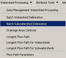
Confirm that the input to the Flow Direction Grid is “Fdr”, and the input to Stream Grid is “Str”. The output Subwatershed is named by default “Subwatershed”, and the output Subwatershed Point is named by default “SubwatershedPoint”.
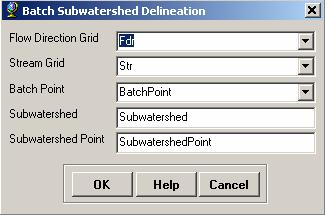
Press OK. The points are added to SubwatershedPoint, and the subwatersheds are added to Subwatershed. The delineated subwatersheds are shown below.
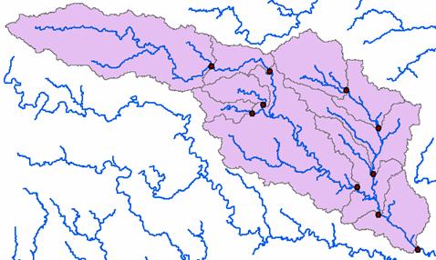
To be
turned in: Make a layout showing the
delineated subwatersheds the
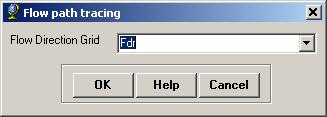
4. Flow Path Tracing
Click on the Flow Path Tracing icon ![]() in the ArcHydro
toolbar to activate the tool. If asked, confirm that the input of the Flow Direction
Grid is “Fdr”.
in the ArcHydro
toolbar to activate the tool. If asked, confirm that the input of the Flow Direction
Grid is “Fdr”.
Click your mouse at any point to determine the flow path. The flow path defines the path of flow from the selected point to the outlet of the catchment following the steepest descent. If you select a point along the stream network, the flow path will follow the exact path of the stream.
To be turned in: Make
a layout showing the flow path for your selected point including the
DrainageLine and the Catchments.
OK. You are done!
Summary
of Items to turn in
1.
Cell size, Number of rows and columns of smdem,
maximum and minimum elevation values in smdem.
2.
Layout with a depiction of topography either
with contours or hillshade in nice colors. Include the streams from NHD. Mark
your point of highest elevation and indicate its elevation.
3.
Make a screen capture of the attribute table of
Fdr and give an interpretation for the values in the Value field using a
sketch.
4.
Report the
drainage area of the
5. A layout with a comparison of the generated
DrainageLine and the NHD river network for
6. How many DrainagePoints, DrainageLines and
Catchments are there? What is the ID
field in each feature class that associates the appropriate DrainagePoint with
its DrainageLine and Catchment? Make a
graphic showing how one associated DrainagePoint, DrainageLine and Catchment
are related.
7. Report the drainage area of the
8. Layout
showing the delineated watershed for your selected outlet. Report the Drainage
Area of the watershed you delineated in km2.
9. Layout
showing the delineated watershed for each USGS Gauging Station. Label each watershed outlet with its
contributing Drainage Area obtained from the Watershed Feature class. Prepare a table using Excel giving Name, USGS
gage number, Watershed point HydroID, Watershed HydroID, Drainage area from
ArcGIS (converted km2).
10. Layout
showing the delineated watershed for your selected point including the
DrainageLine and the Catchments.
11. Layout
showing the delineated subwatersheds the
12. Layout
showing the flow path for your selected point including the DrainageLine and
the Catchments.
Appendix. Procedures for correcting problems with vector processing due to X/Y domain problems.
(Hopefully you do not have to read this.) In previous years problems sometimes occurred due to the X/Y domain of the feature dataset that Arc Hydro created being insufficient to contain all the datasets created. One property of a feature dataset is its X/Y domain. A feature dataset can not hold data outside of its X/Y domain. This problem resulted in not all catchment polygons being created and problems in subsequent processing that used catchment polygons (specifically adjoint catchment processing). This problem is supposed to have been corrected in the latest versions of Arc Hydro, however if this problem occurs this appendix helps you correct the problem.
If you get errors due to an insufficient X/Y domain you will need to use ArcCatalog to delete the feature data set that has insufficient X/Y domain. Usually this feature dataset is named "Layers". Once this is deleted use one of the workarounds below to create a feature dataset with sufficient domain.
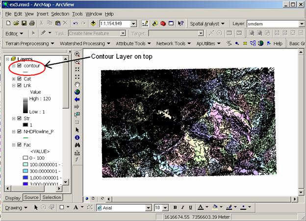
When the first function that creates vector information is executed it creates the "Layers" feature dataset. The feature dataset created by Catchment Polygon Processing in some cases inherits the extent from the top layer in the ArcMap document display. Therefore the chance for X/Y domain problems can be reduced by having the top layer be one that occupies the full extent needed. In the illustration below the "contours" shapefile feature class is on top to provide an extent for the X/Y domain, when the Catchment Polygon Processing function is run.
If having a layer with large extent on top does not work the problem can also be avoided, more tediously, by manually creating a feature dataset named layers within the geodatabase with sufficient X/Y domain prior to running Catchment Polygon Processing as described below.
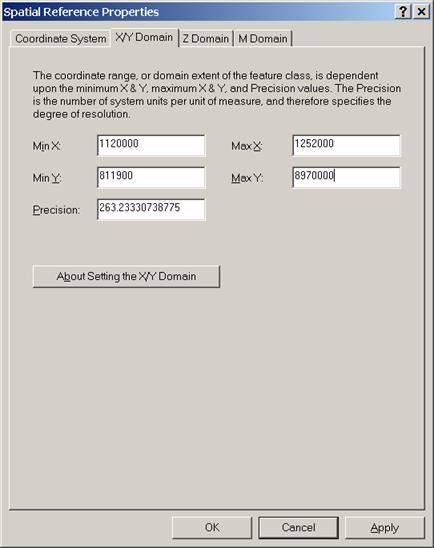
1 First use the pointer in ArcMap to note X/Y domain coordinates that cover the entire domain of the DEM (xmin: 1120000, xmax: 1252000, ymin: 811900, ymax: 897000 in this case).
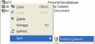
2. Close ArcMap and open ArcCatalog. Right click on the personal geodatabase associated with your map document (ex3, inheriting the name from the map document). If the feature dataset "Layers" is present, delete it. Next create a New Feature Dataset.
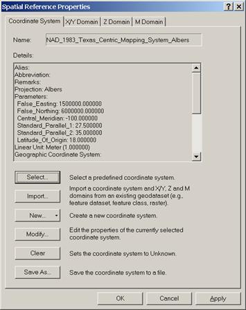
Specify the name "Layers" and click on Edit to edit the spatial reference
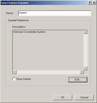
Click Select and browse to the desired projection (NAD_1983_Texas_Centric_Mapping_System_Albers).
Click on X/Y Domain and set the bounds to the values noted above
Click OK twice to create the "Layers" feature dataset. Close ArcCatalog.