GIS in Water Resources
Fall 2005
Goal
The goal of this exercise is to serve as an introduction to Spatial Analysis with ArcGIS.
Objectives
· Calculate slope from a grid digital elevation model
· Apply model builder geoprocessing capability to program a sequence of ArcGIS functions
·
Use raster data and raster calculator
functionality to perform calculations of flooded area and flood volume due to
the Hurricane Katrina flooding of
Computer and Data
Requirements
To carry out this
exercise, you need to have a computer, which runs the ArcInfo version of ArcGIS. The necessary data are provided in the
accompanying zip file, Ex3.zip.
Part 1. Slope
calculations
1.1 Hand
Calculations
Given the following grid of elevations. Calculate by hand the slope and aspect (slope direction) at the grid cell labeled A using
(i) The standard slope function
(ii) The 8 direction pour point model
(iii) The D¥ algorithm
Refer to the powerpoint slides from lecture 6 to obtain the necessary formulas for each of these methods
Grid cell size 100m
|
57 |
55 |
47 |
48 |
48 |
|
53 |
67 |
56 A |
49 |
52 |
|
53 |
52 |
45 B |
42 |
43 |
|
51 |
58 |
40 |
41 |
40 |
Comment on the differences and indicate which you think is a most reasonable approximation of the direction of water flow over the surface.
To turn in:
Hand calculations of slope at point A using each of the three methods
and comments on the differences.
1.2 Verifying calculations using ArcGIS
Verify the calculations in (1.1) using ArcGIS Hydro and Geoprocessing functions and TauDEM.
Save the following to a text file 'elev.txt' (This file is also included in Ex3.zip or may be downloaded)
ncols 5
nrows 4
xllcorner 0
yllcorner 0
cellsize 100
NODATA_value -9999
57 55 47 48 48
53 67 56 49 52
53 52 45 42 43
51 58 40 41 40
This shows how raw grid data can be represented in a format that ArcGIS can import.
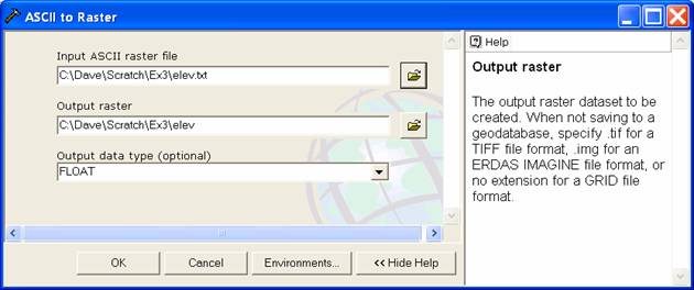
Open ArcMap and ArcToolbox. Use the tool Conversion Tools à To Raster à ASCII to Raster to import this grid file into ArcMap. Specify a name and location for the Output raster (elev) and specify the Output data type as FLOAT (It is more consistent to think of elevation data as including floating point data, rather than integer, even though this specific case is integer data).
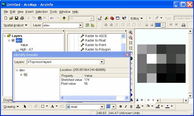
You can use the identify button on the grid created to verify that the numbers correspond to the values in the table above.
![]()
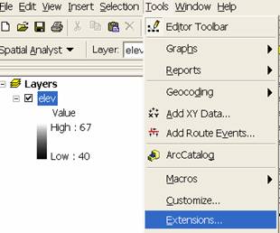
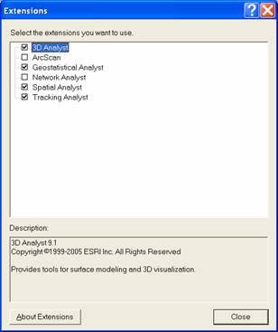
Open Tools à Extensions and verify that the Spatial Analyst function is available and checked. This is where the spatial analyst license is accessed, so if Spatial Analyst does not appear you need to acquire the appropriate license ($$$).
|
|
|
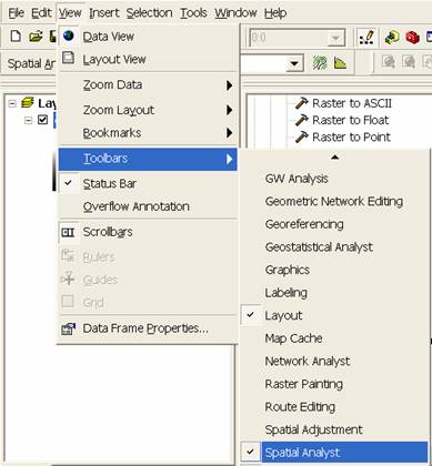
Select View à Toolbars à
Spatial Analyst. This displays the
Spatial Analyst toolbar in the ArcMap interface. You may dock the toolbar somewhere
convenient.
Select Spatial Analyst à
Surface Analysis à Slope on the
Spatial Analyst toolbar.
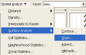
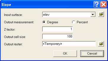
At the dialog that appears select elev as the input surface and select whether you want the output in Degree or Percent (to be consistent with your hand calculations above).
Use the identify button on the slope grid that is created to verify that the numbers correspond to the values you calculated by hand and resolve or reconcile any differences. Record in a table the ArcGIS calculated slope at grid cells A and B (B being the grid cell immediately below A as indicated on page 1)
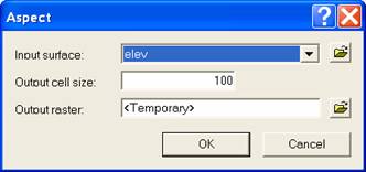
Select Spatial Analyst à Surface Analysis à Aspect on the Spatial Analyst toolbar. At the dialog that appears select elev as the input surface.
Use the identify button on the aspect grid that is created to verify that the numbers correspond to the values you calculated by hand and resolve or reconcile any differences. Record in a table the ArcGIS calculated aspect at grid cells A and B.
Open the Toolbox. Open the tool Spatial Analyst Tools à Hydrology à Flow Direction
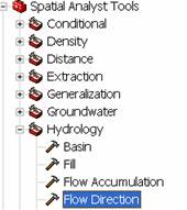
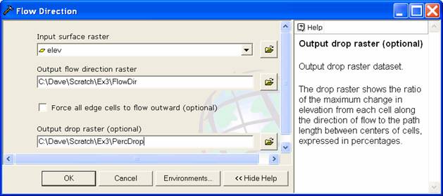
Select elev as the input raster and specify names for output rasters (e.g. FlowDir and PercDrop). Note that raster file names can not exceed 13 characters and that there should not be a space in the name or the file path leading up to the name. Also note that when you click on each field in the dialog box the help part of the dialog to the right explains the content of the file. This is shown below for the Output drop raster which from the description is really the slope expressed as a percentage.
Use the identify button on the FlowDir and PercDrop grids that are created to verify that the numbers correspond to the values you calculated by hand and resolve or reconcile any differences. Record in a table the ArcGIS calculated flow direction and hydrologic slope (Output drop) at grid cells A and B
The D¥ algorithm is not part of standard ArcGIS. Rather it is part of TauDEM that is distributed by as a toolbar plugin to ArcGIS. The TauDEM software is available from http://www.engineering.usu.edu/dtarb/taudem/. Download the setup file and install it.
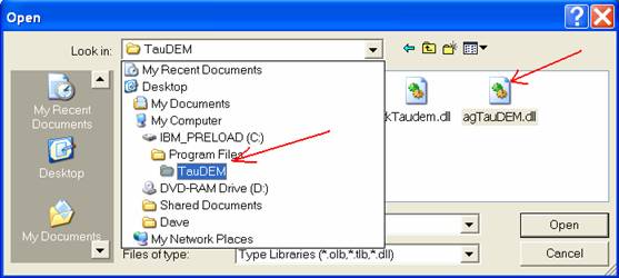
Open ArcMAP and add the TauDEM toolbar. [Click on Tools à Customize à Add from file and select the file c:\program files\Taudem\agtaudem.dll]
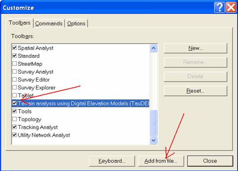
You should get a toolbar that looks like
![]()
This may be docked in a convenient location.
On the TauDEM toolbar select Basic Grid Analysis à Dinf Flow Directions.
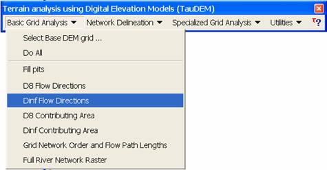
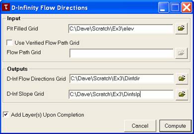
This is the function that computes slope and flow direction using the D¥ method. At the dialog box that appears click on the folder browse button next to the Pit Filled Grid field and browse to the 'elev' grid. Click on the other browse buttons to fill in output names (e.g. DinfDir and Dinfslp, remaining cognizant of the 13 character and no space file name limitations). You do not need to fill in the Flow Path Grid field as we are not using an existing flow path grid. Click compute. This is the only TauDEM function needed for this exercise. We will use other TauDEM functions later in the class.
Use the identify button on the Dinfdir and Dinfslp grids that are created to verify that the numbers correspond to the values you calculated by hand and resolve or reconcile any differences. Record in a table the TauDEM calculated Dinfdir and Dinfslp at grid cells A and B. Note that TauDEM does not compute values for the edges of the domain, because results there are ambiguous due to the data outside the domain not being present, so TauDEM grids will appear smaller. This is not an error.
To turn in:
Table giving slope, aspect, hydrologic slope, flow direction, D¥
slope, D¥ flow direction at grid cells A and B. Please also turn in a diagram or sketch that
defines or indicates what each of these numbers means for the specific values
obtained for cells A and B.
1.3 Automating procedures
using Modelbuilder.
Modelbuilder provides a convenient way to automate and combine together geoprocessing tools in ArcToolbox. Here we will develop a Modelbuilder tool to automate the importing of the ASCII grid and calculation of Slope, Aspect, Hydrologic Slope and Flow direction.
Right click on the whitespace within the ArcToolbox window and select New Toolbox. Name the toolbox "Ex3" (or something else you might like).

The toolboxes created in this manner are stored within the Documents and Settings folder for the user of the computer (e.g. 'C:\Documents and Settings\dtarb\Application Data\ESRI\ArcToolbox\My Toolboxes').
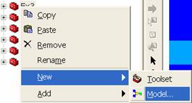
Right-click on the new toolbox and select new model.
The model window should open. This is a window where you can drag, drop and link tools in a visual way much like constructing a flow chart.
In the Toolbox window browse to Conversion Tools à To Raster à ASCII to Raster. Drag this tool onto the model window.
Double click on the ASCII to Raster rectangle to set this tool's properties.
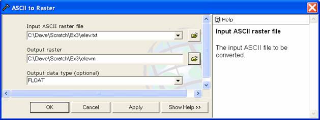
Set the Input ASCII raster file to elev.txt and Output raster to some name (I used elevm so as not to conflict with elev that already exists). Set the output data type to be FLOAT. Click OK to dismiss this dialog. The model elements on the diagram are now colored indicating that their inputs are complete.
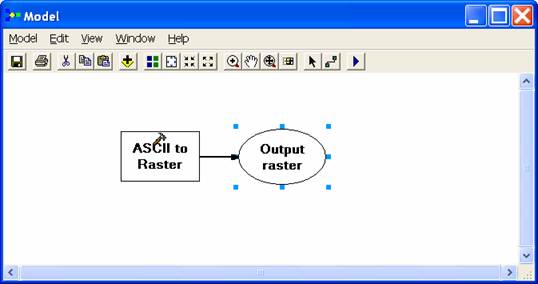
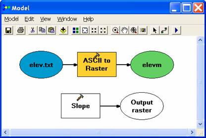
Locate the tool Spatial Analyst Tools à Surface à Slope and drag it on to your window. Your window should appear as follows.
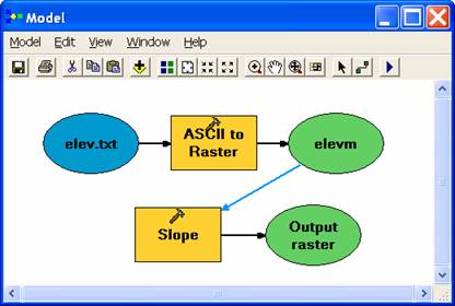
The output from the
ASCII to raster function needs to be taken as input to the slope function. To do this use the connection tool ![]() and draw a line from elevm, the Output raster
of ASCII to Raster, to Slope. Right
click on Output Raster and select 'Add to Display'.
and draw a line from elevm, the Output raster
of ASCII to Raster, to Slope. Right
click on Output Raster and select 'Add to Display'.

You could also
double click on Output raster or slope to change the name of the output file if
you wish (but this is not essential). The
model is now ready to run. Run the model
by clicking on the run button ![]() .
.
![]()
The orange boxes briefly flash red as each step is executed and then the Slope Output raster is added to the Map display.
Add the following two tools
Spatial Analyst Tools à
Surface à Aspect
Spatial Analyst Tools à
Hydrology à Flow Direction
Connect the elevm
outputs to these tools. Use the layout
tool ![]() to organize the layout.
to organize the layout.
Your final model should look something like:
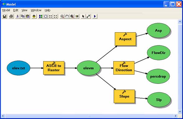
You can click run and do all the processing required to import the data, compute Slope, Aspect, Flow Direction and Hydrologic Slope at the click of a button. Pretty slick!
Right click on elev.txt and select Model Parameter.
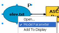
Right click on each of the outputs Asp, FlowDir, Percdrop and Slp in turn and select Model Parameter and Add to Display.
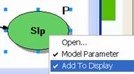
A P now appears next to these elements in the diagram indicating that they are 'parameters' of the model that may be adjusted at run time.
Close your model and click Yes at the prompt to save it. Right click on the model in the Toolbox window to rename it something you like (e.g. SlopeAspect). You are done creating this model. Close ArcMap.
To turn in:
A screen grab of your final model builder model.
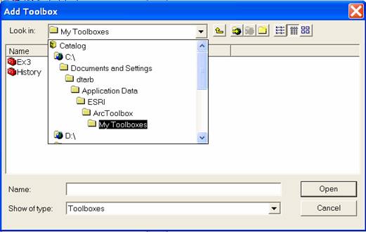
We will now use this model for different data. Locate the file demo.asc within the zip file of data for this exercise. Reopen ArcMap. Right click within the Toolbox area and select Add Toolbox. Browse to the My Toolboxes folder within Documents and Settings for the user of the computer (e.g. 'C:\Documents and Settings\dtarb\Application Data\ESRI\ArcToolbox\My Toolboxes') to locate and add the Toolbox Ex3 that contains the tool you just created.
Double click on the model in the Toolbox window to run it. The following dialog box for the tool you created should appear.

Select as input
under elev.txt the file demo.asc. Specify different names for the outputs Asp,
FlowDir, Percdrop and Slp to avoid the conflicts with existing data and remove
the red crosses ![]() . Then click OK and the model should run and add
results for this new data to ArcMap.
Examine the ArcMap table of contents and record the minimum and maximum
values associated with each of the outputs Aspect, Slope, Flow Direction and
Hydrologic Slope (percentage drop).
. Then click OK and the model should run and add
results for this new data to ArcMap.
Examine the ArcMap table of contents and record the minimum and maximum
values associated with each of the outputs Aspect, Slope, Flow Direction and
Hydrologic Slope (percentage drop).
To turn in:
A table giving the minimum and maximum values of Aspect, Slope, Flow
Direction and Hydrologic Slope (Percentage drop) for the digital elevation
model in demo.asc.
Congratulations, you have just built a Model Builder geoprocessing program and used it to repeat your work for a different (and much larger) dataset.
Part
2. New
Orleans
High resolution elevation
data has been used by the USGS EROS data center to map and estimate inundated
area and the volume of flood water in
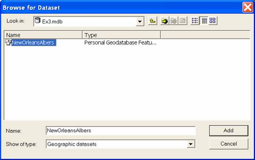
1. Open ArcMap and from the geodatabase Ex3.mdb load the NewOrleans and Water feature classes from the NewOrleansAlbers feature dataset created in Exercise 1. We will work this part of the exercise in the USA Contiguous Albers Equal Area Conic USGS projection that is associated with this feature dataset.
2. Add the grid nedno (National Elevation Dataset New Orleans) to ArcMap. This is a digital elevation model (DEM) of
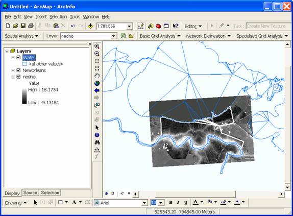
The DEM grid is skewed in this display because it was obtained in geographic coordinates. Right click on the nedno layer in the table of contents and select properties. Click on the source tab. This shows you the Cell Size and number of columns and rows. If you scroll down in the properties you also see the Extent and Spatial reference of this DEM.
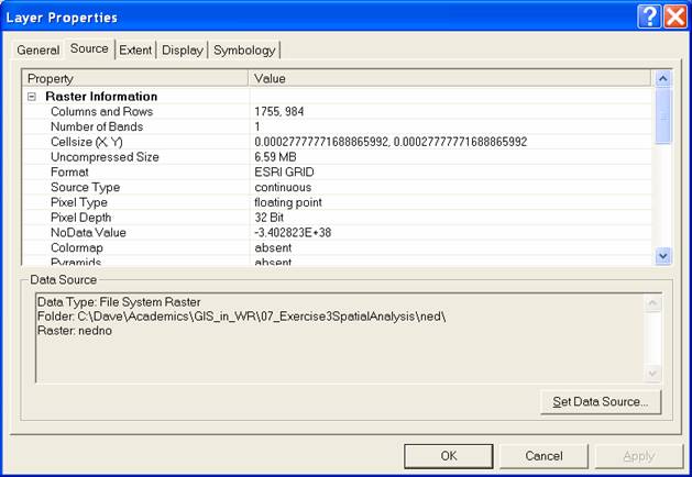
The cell size is in degrees. This is not a very useful measure at this scale. Use what you learned in the lecture on Geodesy to calculate the cell size in m in both the E-W and N-S directions, assuming a spherical earth with radius 6370 km.
To turn in:
The number of columns and rows, cell size in the E-W and N-S directions
in m, extent (in degrees) and spatial reference information for the New Orleans
national elevation dataset DEM 'nedno'.
3. Projecting the DEM. To perform area and volume calculations we need to work with this DEM projected into the Albers equal area projection (An equal area projection is most appropriate for area calculations such as we will be performing). Open the Toolbox and open the tool Data Management Tools à Projections and Transformations à Raster à Project Raster. Set the inputs as follows:
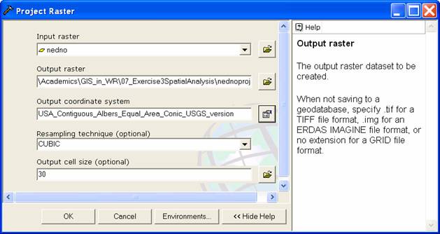
The output coordinate system can be specified using 'Import a coordinate system from an existing data source' after clicking on the button to the right of Output coordinate system'. Then browse to the NewOrleansAlbers feature dataset. This ensures that the projection of the DEM is the same as the other data.
The cell size should be specified as 30 m and cubic interpolation used. I have found cubic interpolation to be preferable to nearest neighbor interpolation for continuous datasets such as DEMs.
Examine the properties of the projected dataset.
To turn in:
The number of columns and rows in the projected DEM. The minimum and maximum elevations in the
projected DEM. Explain why the minimum
and maximum elevations are different from the minimum and maximum elevations in
the original DEM.
4.
Masking the extent. For the
purposes of this exercise we will assume that
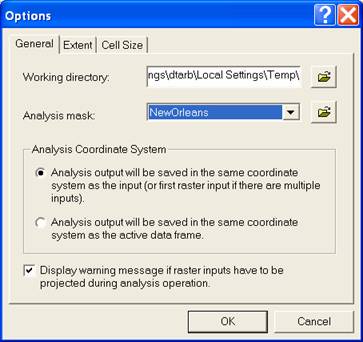
Remove the unprojected 'nedno' DEM from your map document. Select Spatial Analyst à Options and under the General tab set the Analysis mask to the NewOrleans feature class.
|
|
|
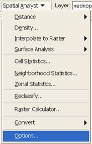
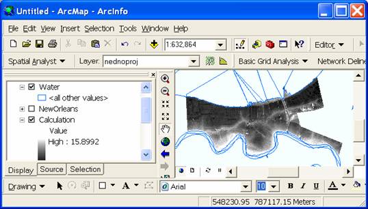
Select Spatial Analyst à Raster Calculator. In the Raster Calculator window double click on the layer nednoproj. One can build complex algebraic expressions using this interface. Here we will initially use a simple expression that is simply the elevations themselves but within the analysis mask. Click Evaluate.

A new grid should
be calculated and added to your map.
Note that this is limited in spatial extent to be within
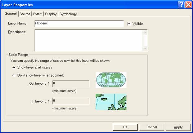
Let's save this DEM for further work. Right click on the layer "calculation" and select "Make Permanent". Provide a name 'NOdem' for New Orleans DEM. Right click on the layer "calculation" and select properties. Under the General tab change the Layer name to NOdem for consistency.
5. Extent of flooded area. Let's find the extent of area below sea level within this DEM. Select Spatial Analyst à Raster Calculator. In the Raster Calculator window construct the expression [NOdem] < 0 by double clicking NOdem then clicking < and 0. Click Evaluate.
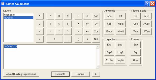
In the calculation grid that appears the elevations less than zero are indicated by 1.
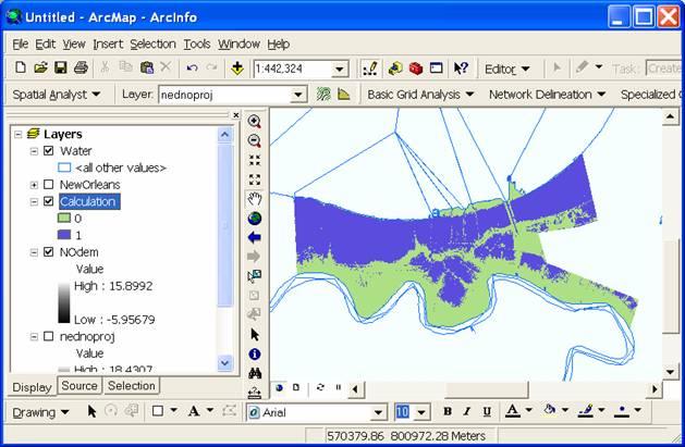
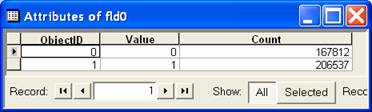
Let's name this flood extent 0, or fld0. Use make permanent to save this as fld0 and Layer properties to label the layer fld0 as before. If we open the attribute table of fld0 (Right click fld0 à Open attribute table) we see that there are 206537 flooded grid cells.
This corresponds to an area of 206537 x 30 x 30 = 185.8 x 10⁶ m2. This is 185 km2 or 72 mi2, incredibly catastrophic (although examining the USGS analysis the dykes did not fail for this entire area so the actual area of flooding is less).
6. Depth of flooded area. The depth of flooding can be calculated by evaluating 0-NOdem within the flooded area. We use the following Raster Calculator expression: (0 - [NOdem]) / [fld0]. The divide by fld0 ensures a result of no data (divide by 0) outside the flooded area. Let's name this result dep0 using make permanent and layer properties to label the layer as before. Adjust the display color scheme to be illustrative of flood depth.
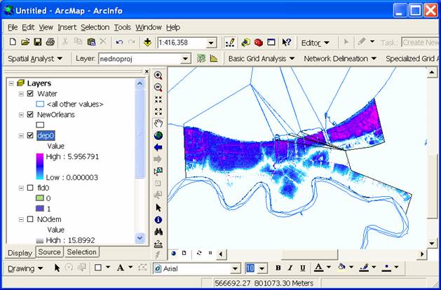
Examine the layer properties of dep0. These show the Minimum, Mean and Maximum flood depth.

Given the mean depth of 1.27 m and the area of 185.8 x 10⁶ m2, the volume of floodwater in New Orleans can be calculated to be 235.97 x 10 6 m3. For those not comfortable with SI units there are 0.3048 m/ft and 4047 m2/acre, so the flood volume is 235.97 x 10 6 /(4047 x 0.3048) = 191.3 x 10³ acre-feet.
To turn in. A map layout showing the depth of flooding
over New Orleans assuming flooding up to Sea Level (zero elevation).
7. Flood Volume and Area Curve. Next repeat steps 5 and 6 for a sequence of
floodwater levels ranging from sea level down to the deepest point in
[NOdem] < -1 (Name the result fld1)
(-1 - [NOdem]) / [fld1]. (Name the result dep1).
This gives the extent of flooded area once the floodwater has been lowered (by pumping) to a -1 m level and the volume of floodwater remaining.
In general
[NOdem] < -z
(-z - [NOdem]) / [fldz].
gives the grids from which you can evaluate the extent of flooded area and volume of floodwater remaining when the floodwater is at level –z.
To turn in. A graph of Flooded area and Flood volume
versus surface water level over the range of z from 0 to -6 m. (If you prefer to work in American units,
i.e. feet, you can do this over the range of z from 0 to -18 ft but there are
18 foot increments and only 6 m increments, so it is more work.)
Summary
of Items to turn in:
1. Hand calculations of slope at point A using
each of the three methods and comments on the differences.
2. Table giving slope, aspect, hydrologic slope,
flow direction, D¥
slope, D¥ flow direction at grid
cells A and B. Please also turn in a
diagram or sketch that defines or indicates what each of these numbers means
for the specific values obtained for cells A and B.
3. A screen grab of your final model builder model.
4. A table giving the minimum and maximum values
of Aspect, Slope, Flow Direction and Hydrologic Slope (Percentage drop) for the
digital elevation model in demo.asc.
5. The number of columns and rows, cell size in
the E-W and N-S directions in m, extent (in degrees) and spatial reference
information for the New Orleans national elevation dataset DEM 'nedno'.
6. The number of columns and rows in the
projected DEM. The minimum and maximum
elevations in the projected DEM. Explain
why the minimum and maximum elevations are different from the minimum and
maximum elevations in the original DEM.
7. A map layout showing the depth of flooding
over New Orleans assuming flooding up to Sea Level (zero elevation).
8. A graph of Flooded area and Flood volume
versus surface water level over the range of z from 0 to -6 m.