Exercise 2. Building a Base Map
CE 394K GIS in Water
Resources
University of Texas
Fall 2005
Prepared by David R. Maidment, Kristina Schneider, and Oscar Robayo
- Goals of the Exercise
- Computer and Data Requirements
- Procedure for the Assignment
- Creating a Geodatabase
- Get Stream and Watershed Data for Water Resources Region 12
- Importing Data in the Geodatabase
- Projecting the Geodatabase
- Selecting the Guadalupe Basin Watersheds
- Getting the Guadalupe River Reaches
- Creating a Point Feature Class of Stream Gages
- Add Attributes to the Point Feature Class
- Creating a Chart and Layout
- Overlaying the Edwards Aquifer
- Adding Data from the Internet
- Downloading USGS Flow Data
Goals of the Exercise
This exercise is intended for you to build a base map of geographic and
streamflow data for a watershed using the
Computer and Data Requirements
To complete this exercise, you'll need to run ArcGIS 9.1 from a PC.
The HUC boundaries are a subdivision of the
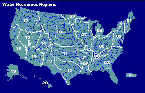
The HUC and RF1 coverages for the
Hydrologic Cataloging Unit
description http://water.usgs.gov/GIS/huc.html
Get the HUC coverages by 2-digit water resource region http://water.usgs.gov/lookup/getspatial?huc250k
Enhanced River Reach File 1
http://water.usgs.gov/lookup/getspatial?erf1
Get the RF1 data by two-digit water resource region ftp://water.usgs.gov/pub/dsdl/
It seems that using Wsftp to ftp://water.usgs.gov/pub/dsdl/ works a lot faster for downloading data than trying to do it through a web browser.
Procedure for the Assignment
Logon to the computer of your choice and make a directory in your workspace for this exercise. I've saved the needed files in the LRC class directory (Civil5/LRC/Class/Maidment/giswr/guadalupe/). They may also be downloaded as Guadalupe.zip
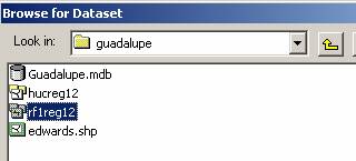
Unzip the files to get the following:
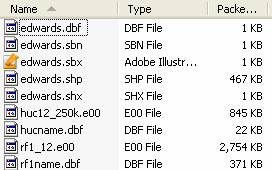
The HUC12 and RF1 files are coverages stored in Arc/Info interchange file format as indicated by the .e00 so you will need to import them using the Import from Interchange file tool in ArcToolbox as you will learn. The Rf1name.dbf and hucname.dbf are tables with name information for your streams and watersheds.
Get the Stream and Watershed Data for Water Resources Region 12
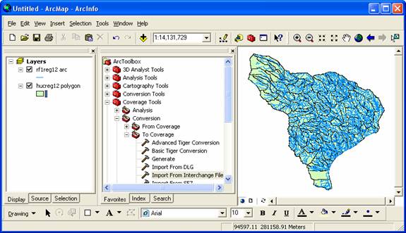
(1) Open ArcMap (Start à Program Files à ArcGIS à ArcMap)
(2) Display the ArcToolbox window
by clicking on the ![]() icon.
This will add a new dockable window the ArcMap as shown below.
icon.
This will add a new dockable window the ArcMap as shown below.
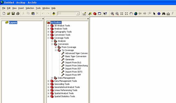
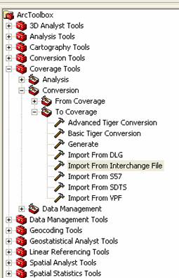
(2) In the ArcToolbox window, select Coverage Tools à Conversion à To Coverage à Import From Interchange File as shown below.
Navigate to the location of the Input file Rf1_12.e00. Then indicate where the output coverage should be located (your data folder) and what it should be called. When importing rf1_12.e00, name the resulting coverage rf1reg12. Be careful to give the full pathname for the Output dataset. Don’t just give the name of the output file and assume that it will be put into the same location as where the input file comes from. If you don’t do this, what will have happen is that the imported coverage will be saved somewhere to a default directory location but you don’t know where it is located.
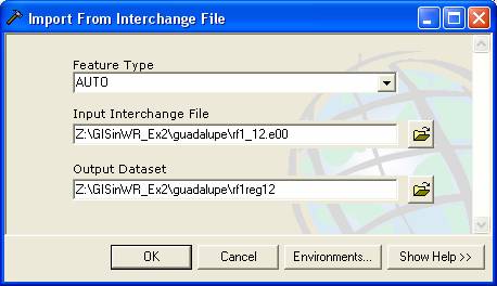
Press OK. Don't worry if processing takes a while, the file is rather large.
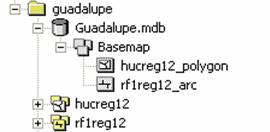
(3) Repeat the process with the huc250k.e00 file. When you import huc_250k.e00, name the resulting coverage hucreg12. This is how the result looks in Windows Explorer.
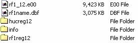
The geospatial data files defining the drainage areas and rivers are in the hucreg12 and rf1reg12 folders, respectively, and the attribute tables for both coverages are in the Info folder. Notice that while the geospatial files for each coverage are held separately, their attribute tables are merged into single Info folder. This means that whenever you wish to copy coverages from one place to another in your workspace, you need to use the Arc Catalog Edit/Copy to copy the coverage rather than just using Copy in Windows Explorer.
If you look inside the rf1reg12 folder, you’ll see the following. The Arc.adf file is where the geometry file for the coverage is stored. The prj.adf file is the projection of this coverage.
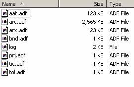
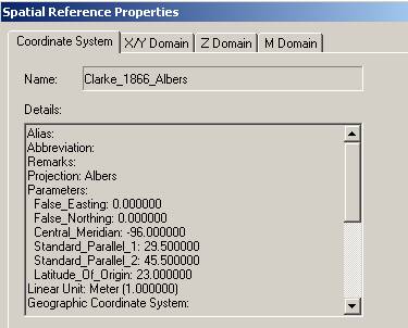
You can open the prj.adf file with a Word processor to see the
projection. This is the USGS National
Albers projection, a standard for USGS data of the
Projection ALBERS
Zunits NO
Units METERS
Spheroid CLARKE1866
Xshift 0.0000000000
Yshift 0.0000000000
Parameters
29 30
0.000 /* 1st standard parallel
45 30
0.000 /* 2nd standard parallel
-96 0
0.000 /* central meridian
23
0 0.000 /* latitude of
projection's origin
0.00000
/* false easting (meters)
0.00000 /* false northing (meters)
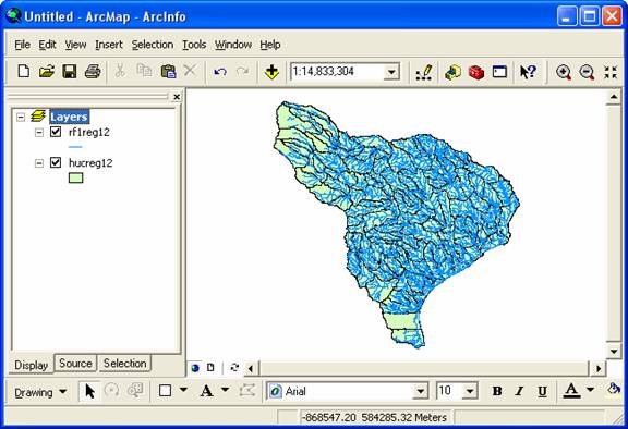
Add the two coverages to Arc Map using the ![]() button:
button:
Recolor the themes if you wish.
Move the cursor to the lower left corner of the display, and you’ll see
the coordinates changing at the bottom of the map display. The ones shown here at (–889403, 288539),
which means that point is 889.4 km to the West and 288.5 km to the North of the
coordinate origin, which is (0,0) at 23 ºN and 96 ºW in
this projection). If you move the cursor
to the upper right of the display, you’ll get a different set of coordinate
points. I got (521560, 1360524), which
means that the upper right location is 521.6km to the East and 1360.5 km to the
North of the coordinate origin. The
change from negative to positive on the Easting coordinate between these two
points is because the central meridian of this projection (96ºW) runs through the middle of
We’ll use this projection information and these bounding points to create a reference frame for these data.
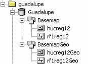
ArcInfo 8 introduced an object-oriented data model called the geodatabase data model. This data model gives the features in your GIS datasets custom behaviors and the possibility to create relationships between features. In general, a geodatabase model provides a standardized framework into which various types of data can be loaded. Once created, the geodatabase is a Microsoft Access file called an ArcGIS personal geodatabase.
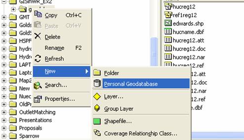
Close ArcMap (you don’t have to save the map document) and open ArcCatalog. Right click on the data folder, press New / Personal Geodatabase. Call the new geodatabase Guadalupe.
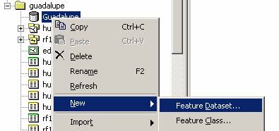
Right click on the geodatabase, and select New Feature Dataset.
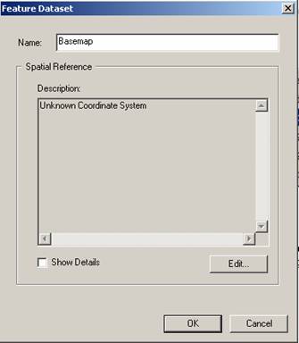
Name the new feature dataset Basemap, and select Edit to set the projection and map extent.
We will import the coordinate system from the prj file of the rf1reg12 coverage. Select Import from the choices in the menu displayed
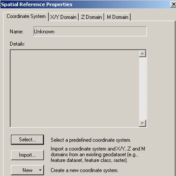
You’ll see that the coordinate system is now specified:
We’ll enter the X/Y domain definition from the coordinates that we found earlier in Arc Map: (MinX, MinY) = (–889403, 288539), (MaxX, MaxY) = (521560, 1360524). The precision is calculated for you and should equal what is shown below.

Hit Apply and Ok, to finish setting the Spatial Reference
Frame of the Feature Dataset.
Importing data into the Geodatabase
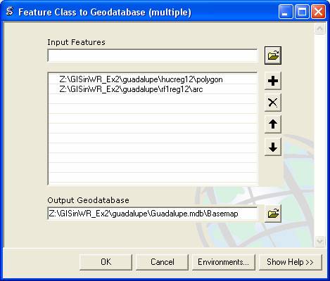
(1) Now, you will import the created coverages for the Region 12 into the Guadalupe geodatabase. Right-click on your feature dataset and press Import à Feature Class (multiple)… as shown below.
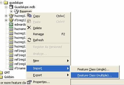
You will be importing the two existing coverages, hucreg12 and rflreg12, into the feature dataset Basemap of the geodatabase Guadalupe. Browse to hucreg12 and add its polygons. Then browse to rf1reg12 and add its arcs (as shown below).
Here is the new feature dataset that you’ve just created with its two new feature classes included:
Rename the feature classes by right-clicking on each. Change hucreg12_polygon to hucreg12 and rf1reg12_arc to rf1reg12.
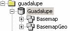
Projecting the Geodatabase
We’ll now project these data into geographic
coordinates. Establish a new feature
dataset called BasemapGeo. Follow the same procedure as before for the
Basemap feature dataset, except that when you are setting the coordinate
system, use Select and
you’ll see the following choices appear:

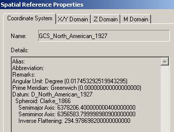
Select the Geographic Coordinate
Systems and North
American Datum 1927.

Hit apply and Ok and now you’ve got two feature
datasets, one in Albers projection and one in geographic coordinates.
Now lets export the feature classes to the
geographic feature dataset. Go to the
Basemap feature dataset and right click on the hucreg12 feature class and
select Export à To Geodatabase (single)…
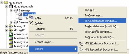
Select the BasemapGeo
feature dataset as the output location and hucreg12Geo as the
output feature class name.
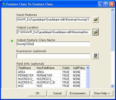
Do the same for to export the Rf1reg12 from Basemap to Rf1reg12Geo
in BasemapGeo. You now have two feature datasets, one for each
coordinate system:
If you right click on BasemapGeo and go to
Properties, and then selected Edit, you’ll see the new coordinate system:
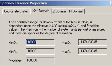
and if you select X/Y Domain, you’ll see that the
range of the coordinate system is automatically set to something outside –180
to 180 in East-West and –90 to 90 North-South, so this range will accept any
data in geographic coordinates for any point on earth.
You cannot change the spatial reference of a feature
dataset once it has been set, so if you make a mistake in this sequence, you
have to start again by establishing a new feature dataset.
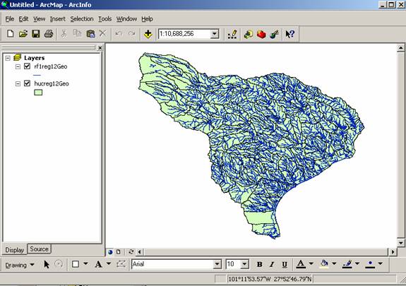
Open ArcMap and display the data in the BasemapGeo
feature dataset. Notice how the cursor
shows Degrees, Minutes and Seconds as you navigate through the display.
To Be Turned In: What is the approximate map extent of these
data in geographic coordinates? Use the
Draw Tools in ArcMap to draw a line on the map showing the Central Meridian of
the projection at 96ºW and another line showing the Standard Parallel at 29º
30’ N. Screen capture the resulting map
display and include it in your solution.
Selecting the Guadalupe Basin
The imported Hucreg12 and Rf1reg12 feature classes cover a large region and
we only want to work in the
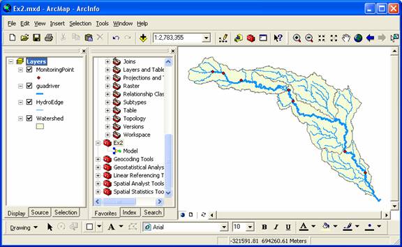
(1) Start up ArcMap and add the Basemap feature dataset to your map document. Recolor the themes as necessary. You can select a symbol font for “River” to color in the blue line rivers.
(2) Use File/Save As to save the ArcMap document as Ex2.mxd (to save your own customized colors).
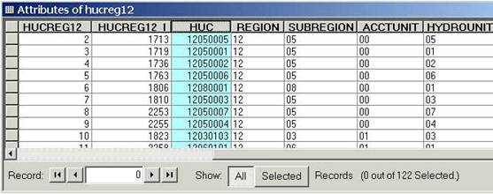
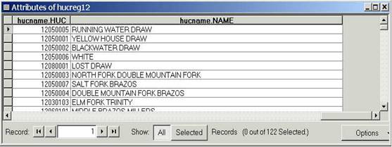
(3) Right click on the hucreg12 theme and select Open Attribute Table to bring up the table of its attributes. Scroll across the fields and see the Hydrologic Unit Code (HUC), Region (first 2 digits of HUC), Subregion (second 2 digits of HUC), Basin (or Accounting Unit) (third 2 digits of HUC) and the Subbasin (or Hydro Unit) (fourth 2 digits of HUC).
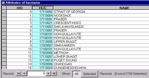
You’ll see that these HUC watersheds are identified by numbers rather than names. We have a separate names file hucname.dbf that was prepared from another HUC coverage that we’ll use to attach names to the HUC polygons.
(5) Hit the Add Data button ![]() and in the dialog box that appears, select the
hucname.dbf table. The table hucname is added to your map. We’ll join this table to the HUC
attributes so that we can identify the HUC watersheds by name. This names file contains the names of all the
2156 HUCs in the continental
and in the dialog box that appears, select the
hucname.dbf table. The table hucname is added to your map. We’ll join this table to the HUC
attributes so that we can identify the HUC watersheds by name. This names file contains the names of all the
2156 HUCs in the continental
(6) Right Click on the hucreg12 layer in Arc Map and select Joins and Relates/Join.... What you are doing here is associating corresponding records in the two tables using HUC as the key field values that they have in common.
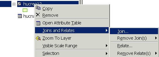
(7) Select the attribute HUC for question 1. For the second question, browse for the hucname.dbf table since it is not a layer in the map and therefore will not be automatically recognized. Again, for the third question select the HUC common attribute. Click OK. (Click No if you are asked to add an index field to the hucname.dbf file)

Voila!! Now we have a Name attribute on the Attributes of Hucreg12 table so that it is easier to understand what river basin we are in.
Lets recolor the HUC’s by subregion to get some sense of the river basin organization within Region 12. You do this using the Symbology tab under layer Properties. Right Click on the layer and select Properties. Under Show in the same box choose select Categories/Unique Values, select hucreg12.SUBREGION as the value field to be symbolized. Finally, press Add all values and OK.
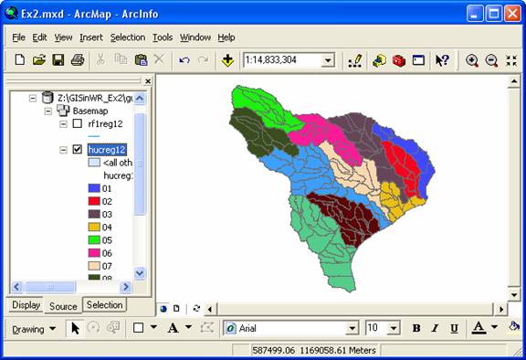
If you use the Information tool ![]() you can click around and get a sense of the
names of the river basins and their subunits.
(8) Use the Select button
you can click around and get a sense of the
names of the river basins and their subunits.
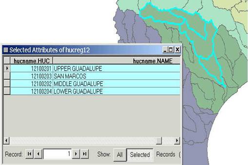
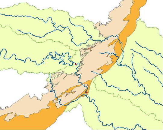
(8) Use the Select button ![]() and visually select the 4 HUC units in the
Guadalupe basin (see image below). Hold
down the shift key so that you can select more than one at a time. Open the layer attribute table and press the
Selected button. This will show you the items you have selected. You will see
that the
and visually select the 4 HUC units in the
Guadalupe basin (see image below). Hold
down the shift key so that you can select more than one at a time. Open the layer attribute table and press the
Selected button. This will show you the items you have selected. You will see
that the
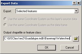
(9) Make sure that Arc Catalog is closed or the next steps won’t work. In ArcMap, Right Click on hucreg12 and select Data/Export Data ... to produce a new theme. If you get a message saying you can’t do this, it means that you haven’t shut down Arc Catalog before trying the data export. Close Arc Catalog and repeat the export steps if this happens.
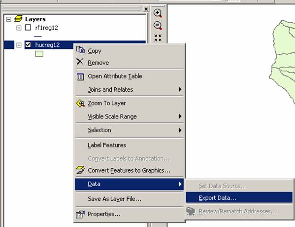
Browse inside your geodatabase to the Basemap Feature dataset (you’ll have to change the Save as Type to Personal Geodatabase feature classes first), name this new feature class as Watershed and save it in the geodatabase as a Personal Geodatabase feature class. Don’t save it as a Shapefile, which is the default option you are first presented with.
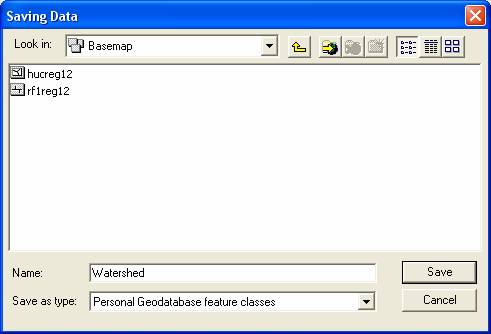
The program will automatically convert only the selected features. Note: By assigning Arc Hydro standard names like Watershed to your feature classes it will be easier to apply the capabilities of the ArcHydro data model as you will see later in this class (See page 32 on Arc Hydro book for standards).
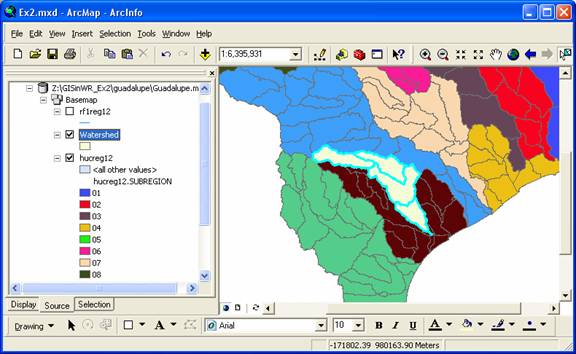
You will be prompted to whether add this theme to the Map, click Yes. Notice the Watershed Feature Class looks identical to the earlier hucreg12 feature class selection for the Guadalupe basin, but the new Watershed class is much smaller. Notice that it carries all the attributes of hucreg12 and the hucname.dbf table that you joined before making the data export.
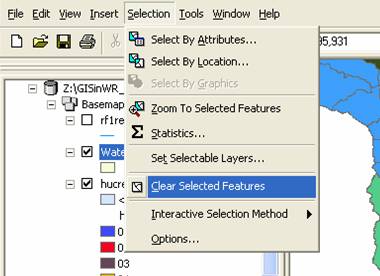
(10) Select Selection à Clear Selected Features to clear the selections you made from Hucreg12.
Getting the Guadalupe River
Now we need to select the rivers in rf1reg12 that
fall within the
(1) In ArcMap, Right Click on the rf1reg12 layer and select Joins and Relates/Join. Select the field RR (River Reach) for question 1. For the second question, browse for the rf1name.dbf table since it is outside of the geodatabase and therefore will not be automatically recognized. Again, for the third question select the RR attribute. Click OK. (Do not add index fields to the table if you are prompted to do so.)
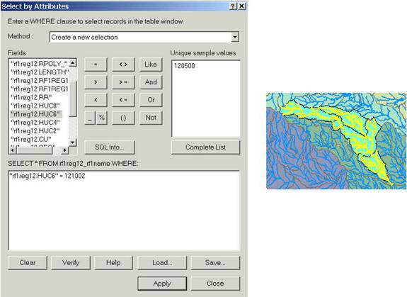
(2) Open the attribute table for the rf1reg12 feature
class. Click on the Options/Select by Attribute and a dialog will
appear. Use the “Create a new selection” Method and double click on the
"rf1reg12.HUC6" field. Set this field equal to 121002 (The
6-digit HUC number for Guadalupe). You'll see that now only
the rivers within the
(3) As we did with the selected HUCs, Right Click on rf1reg12 and select Data/Export Data ... to produce a new feature class out of this selection. Browse inside your geodatabase to the Basemap Feature dataset, name this new feature class as HydroEdge (another standard ArcHydro name) and save it in your geodatabase. You will be prompted to whether add this theme to the Map, click Yes.
(4) Highlight the hucreg12 and rf1reg12 themes in the legend bar (use Shift when highlighting the second theme). Right click and press Remove to delete them from the Map. From now on, we'll work with the HydroEdge and the Watershed Feature Classes that correspond to our area of interest and to save time in displaying the layers.
(5) Once you've got the
(6) Open the HydroEdge attribute table. Scroll across to the names of
the rivers. PNAME is the name of the river segment. Use the Select by Attributes interface to
select "PNAME" = 'GUADALUPE R' and change the table view to the
selected records. This shows the main channel of the
(7) Right click on the HydroEdge Feature Class and use Data/Export
Data to export a new Feature Class with the main channel of the
(8) Click on the symbol boxes to recolor your map to the form you want it in. Make a layout of this map, copy it to the clipboard and paste it to a Word file so you can turn it in.
To be turned in: the layout of the
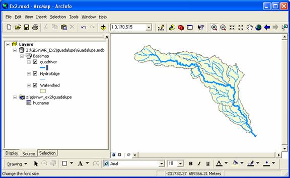
(7) Save your ArcMap document, Ex2.mxd. Exit ArcMap.
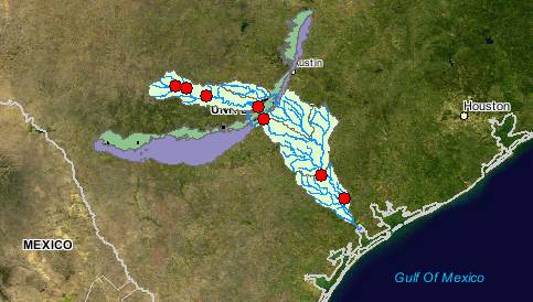
Creating a Point Feature Class of Stream Gages
Now you are going to build a new Feature Class yourself of stream gage
locations on the Guadalupe. I have extracted information from the USGS stream
gage data books information about 7 gages on the main stem of the
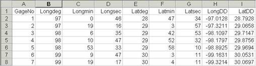
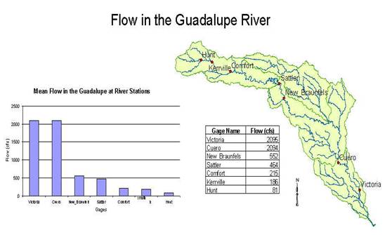
Seq# Station# Name Longitude Latitude Mean Annual Flow (cfs)1 08176500 Victoria 97 00 46 W 28 47 34 N 20952 08175800 Cuero 97 19 16 W 29 03 57 N 2094 3 08168500 New_Braunfels 98 06 35 W 29 42 53 N 552 4 08167800 Sattler 98 10 47 W 29 51 32 N 464 5 08167000 Comfort 98 53 33 W 29 58 10 N 215 6 08166200 Kerrville 99 09 47 W 30 03 11 N 1867 08165500 Hunt 99 19 17 W 30 04 11 N 81
The location coordinates and flow data for each of the gages was obtained from the USGS Water-Data Report TX-92-3. It can also be obtained from the USGS NWIS server, as described subsequently in this exercise.
(a) Define a table containing an ID and the long, lat coordinates of the gages
The
coordinate data is in geographic degrees, minutes, & seconds. These values
need to be converted to digital degrees, so go ahead and perform that
computation for the 7 pairs of longitude and latitude values. This is something
that has to be done carefully because any errors in conversions will result in
the stations lying well away from the
Decimal Degrees (DD) = Degrees + Min/60 + Seconds/3600
Remember that West Longitude is negative in decimal degrees. Shown below is a table that I created. Be sure to format the columns containing the Longitude and Latitude data in decimal degrees (LongDD and LatDD) so that they explicitly have Number format with 4 decimal places using Excel format procedures. Save the file as latlong.dbf as type (DBF4, dBASE IV) in Excel. If you don't explicitly format your decimal degree columns, you'll find that you've lost significant figures after the decimal places when you incorporate the table latlong.dbf into ArcMap. Close Excel before you proceed to ArcMap.
(b) Creating and Projecting a Feature Class of the Gages
(1) Open ArcMap and the Ex2.mxd file you created in the first part of this exercise. Add the latlong.dbf table created in Excel.
(2)
Add the Toolbox window by clicking the ![]() icon.
Right click in the toolbox window and select a new Toolbox. Name the new toolbox “Ex2”.
icon.
Right click in the toolbox window and select a new Toolbox. Name the new toolbox “Ex2”.
(3) Right-click on the new toolbox and select new model.
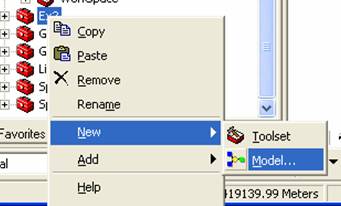
This introduces a new concept in ArcGIS 9 – Model Builder. Model Builder allows you to string together processing routines to create custom models, as you’ll see in this example.
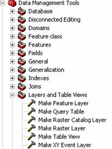
(4) In the Toolbox window browse to Data Management Tools à Layers and Table Views à Make XY Event Layer.
(5) Drag this tool to your new model.
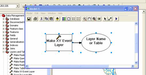
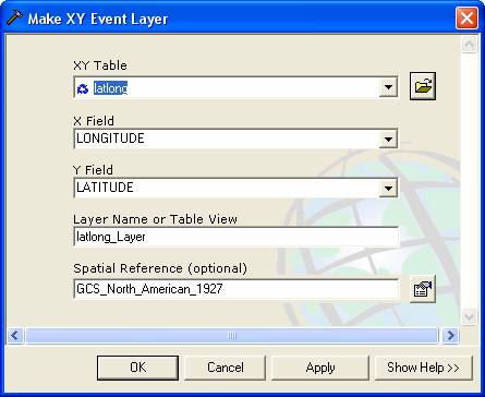
(6) Double-click on the Make XY EventLayer to get the tool’s properties. Set the XY Table to latlong, the X Field to Longitude (or LongDD), the Y Field to Latitude (orLatDD), keep the Layer name as the default, and add the spatial reference of the BasemapGeo feature dataset. Press OK. Notice that the model has color now. This indicates that all of the models parameters are satisfied and the model is ready to run.
Right now the tool reads the latlong.dbf file and creates point events (not actual features) in geographic coordinates. What we need to do is write these point events to the Guadalupe geodatabase a feature class.
(7) In the Toolbox window browse to Data Management Tools à General à Copy. Drag this tool onto your model as we did before.
(8)
Select the ![]() tool. Click on the green latlong_layer oval
and then release the mouse button on the copy features rectangle. This links the output of XY Events tool with
the Copy Tool.
tool. Click on the green latlong_layer oval
and then release the mouse button on the copy features rectangle. This links the output of XY Events tool with
the Copy Tool.
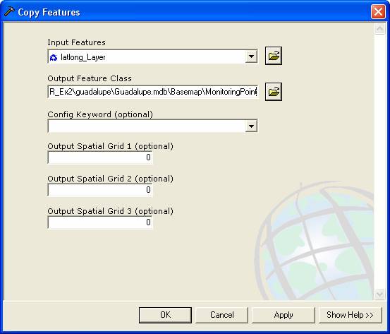
(9) Double-click on the Copy tool to get its properties. Set the output feature class to a new feature class named MonitoringPoint in the feature dataset BaseMap. Press OK.
(10) To add the feature class to the map, right click on the green oval “MonitoringPoint” and select “Add to Display”.
(10) At this point, the model should be colored and ready to run. Go to Model à Run Entire Model to execute the model. You’ll see the model progressing as each tool turns red indicating the current processing step. Press Close once the model is complete. Close the model and save changes.
The Albers projection is done on the fly as this copy tool writes the the Basemap feature dataset. If your gages are in the wrong place, check the latlong.dbf file and make sure it is correct.
(11) Save your Ex2.mxd ArcMap document, and construct a layout to turn in.
To be turned in: a layout or screen capture of the MonitoringPoint attribute table with the map.
Add Attributes to the Point Feature Class
Now we are going to add the USGS gage ID, gage name, and annual discharge for each gage as new attributes in ArcCatalog.
(1) Open ArcCatalog and navigate to the Guadalupe geodatabase that contains your data.
(2) Right click on the MonitoringPoint feature class, and click on Properties to open the Feature Class Properties window. Click on the Fields tab and scroll down to the end of the Field Name list. Type the following three entries:
|
Field
Name |
Data
Type |
|
USGSID |
Text |
|
Name |
Text |
|
Flow |
Long
Integer |
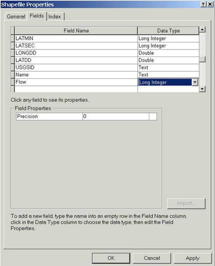
(3) Click OK and open your ArcMap document ex2.mxd.
Adding Data to the Attribute Table
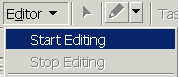
(1) In ArcMap right click on the MonitoringPoint feature class and open the attribute table. Scroll to the right until you see the new fields you have created. Start editing by selecting Editor/Start Editing.
If the Editing Toolbar is not visible it maybe added by selecting View/Toolbars/Editor.

(2) You may now just add the appropriate data values to the table and for the three attribute fields you added. Continue adding the data values until they are all done.
The following data are needed in the table:
Number USGSID Name Flow 1 08176500 Victoria 2 08175800 Cuero 2094 3 08168500 New_Braunfels 552 4 08167800 Sattler 464 5 08167000 Comfort 215 6 08166200 Kerrville 7 08165500 Hunt 81
(3) Select Editor/Stop Editing to finish editing and say Yes when it asks if you would like to save your edits. Note that you can only edit tables for which you have write permission (i.e. your own tables not tables in my work area).
Labeling the Gages in the View
Now you can use the Name field that you've added as a label for the gages.
(1) Right Click on the MonitoringPoint feature class and select Properties. Click on the Label tab and from the drop down menu select the label field to be Name. Click OK.

(2) Right click on the MonitoringPoint feature class again and select “Label Features”. You can now create a view like this:
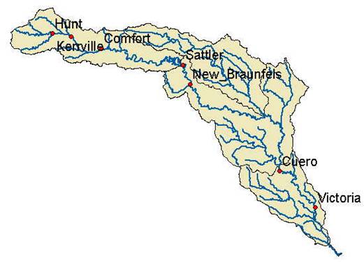
Pretty awesome!
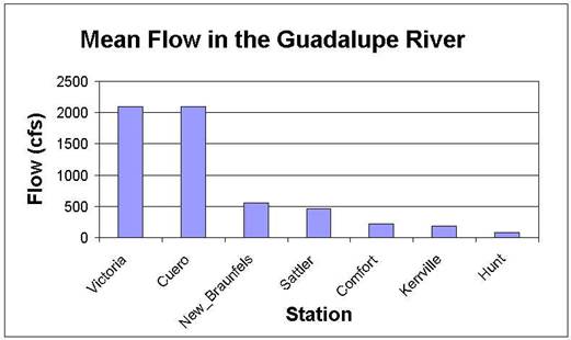
Creating a Chart and Layout
(1) Open ArcMap to create a chart of the mean annual flow of the Guadalupe gages. Open the MonitoringPoint Attributes table file and make a chart using the tools available in ArcMap. Alternatively, you can export the attribute table to a .dbf file and map the chart in Excel. You can also open the geodatabase tables directly in Excel by using Data/Get External Data and doing a query on the Microsoft Access file that contains the geodatbase. The chart may look something like this
(2)
In ArcMap prepare a layout showing a map of the drainage area, the graph
of its annual flows at each gage and a table of numerical values
describing the gages. You can import your Excel chart and worksheet from
the Insert/Object... option in ArcMap. If necessary resize the
original chart or table smaller so that it can be displayed in the layout.
You'll see in the chart that the flow in the
To
be turned in: a layout showing the base map, chart and data table for the
Overlaying the Edwards Aquifer
The
Edwards aquifer is one of the most critical water resources of
The Edwards aquifer coverage from TNRIS is in Decimal Degree coordinates. We are using an Albers projection because it preserves earth area. I projected the Edwards coverage to Albers TSMS coordinates. This is the Edwards shapefile that you copied from the zip file at the beginning of the exercise.
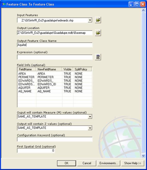
(1) Import your Edwards.shp file into the Guadalupe geodatabase. From the Toolbox window in ArcMap, select Conversion Tools à To Geodatabase à Feature Class to Feature Class. Although the name of the tool is feature class to feature class, it will also convert a shapefile to feature class.
(2) Choose Edwards.shp as the Input Features, the Basemap feature dataset of the Guadalupe geodatabase as the output location, Aquifer as the output feature class name, and leave the rest of the inputs as their default values. Press OK.
This will not only do the conversion from shapefile to feature class, but also add the new feature class to your map.
(3) Right click on the Aquifer feature class and select Properties. Click on its Symbology tab and Label the theme using the attribute Aquifer. This attribute has three values: 1 for outcrop, 2 for downdip and 0 for holes within the outer boundary of the aquifer. Classify the values with Unique Value and color them appropriately.
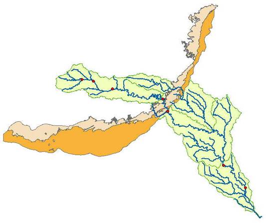
You'll see that as the
To be turned in: Between which two gaging stations does the Edwards aquifer
outcrop area occur? What is the difference in mean annual flow at these two
gages? Comment on these data. Do they seem correct to you?
Adding Data from the Internet
ESRI has
developed a map library service called the Geography
Network which can be accessed to add themes to your map. There are other map services, such as seamless.usgs.gov and geodata.gov from which data can also be
added to your map. Lets use the
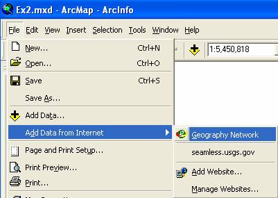
Geography Network to get some satellite imagery. In ArcMap, use File/Add Data from Internet/Geography Network to
access the Geography Network.
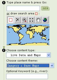
You’ll
see that you are presented with a selection palette with a map of the world and
a series of options for map content.
Leave the content type as Live Data and Maps and Choose Imagery & Base Maps as the content theme.
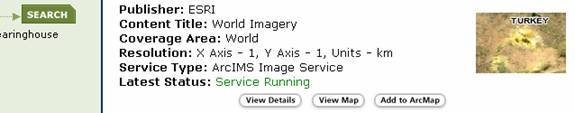
Hit Search and select ESRI World Imagery. Add
it to your map by hitting the Add to
ArcMap button.
And
you’ll see a nice background image of South Texas
appear which provides a sense of context for your study area. Cool!
To be turned in: A map showing map images
added to your basemap information from the Geography Network.
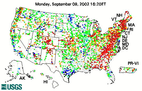
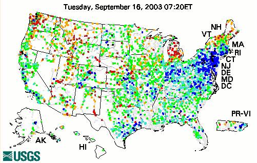
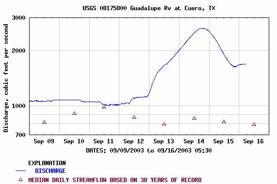
Downloading USGS Flow Data
There are also other sources of flow data. One of them is real time data via Internet from the U.S. Geological Survey (http://water.usgs.gov/realtime.html). This data is taken at the gage sites every 15-60 minutes and is transmitted to the USGS office every 1 to 4 hours. This data relayed using satellite, telephone, and/or radio and can be viewed within minutes on arrival to the office. Notice the difference between the flow conditions in September 2002 (when last we did this exercise) and this September. A year ago, the Northeast was experiencing a severe drought while today it is wetter than normal.
(1) Click on the site http://water.usgs.gov/realtime.html.
(2)
Once you have looked around a bit click on
To
be turned in: The graph of flow of the
Summary
of Items to be Turned in:
1.
A layout of the
2.
What is the approximate map extent of these data in geographic
coordinates? Use the Draw Tools in
ArcMap to draw a line on the map showing the Central Meridian of the projection
at 96ºW and another line showing the Standard Parallel at 29º 30’ N. Screen capture the resulting map display and
include it in your solution.
3.
A layout or screen capture of the MonitoringPoint attribute table with the map.
4.
A layout showing the base map, chart and data table for the
5.
Between which two gaging stations does the Edwards aquifer outcrop area occur?
What is the difference in mean annual flow at these two gages? Comment on these
data. Do they seem correct to you?
6. A map showing map images added to your
basemap information from the Geography Network.
7. The graph of flow of the