Hydrologic Analysis of the
Brad
Wolaver
Dr.
David Maidment, CE 394K, Fall 2004
TABLE OF CONTENTS
3.0...... STREAM NETWORK DELINEATION
4.0...... FRACTURE TREND ANALYSIS
5.0...... CANAL DISCHARGE OUT OF
BASIN
APPENDIX A - Approaches to Filling Null Data Cells in
an STRM DEM
1.0 INTRODUCTION
The Cuatro Ciénegas basin (CCB)
of north‑central Mexico represents a unique groundwater‑dependent
desert aquatic ecosystem comprised of dozens of springs that flow into
permanent streams and lakes in a 200,000‑acre semi‑arid valley
surrounded by 10,000‑ft mountains (Tang and Roopnarine, 2003) (Figure 1). Radiocarbon dating and fossil pollen analysis
of valley sediment collected in cores indicate a stable environment for at
least the past 30,000 years (Meyer, 1973). Although Meyer (1973) asserts that the
highly‑endemic nature of fauna suggests that Cuatro Ciénega’s
special habitat of springs and ponds has existed since the early Tertiary or
late Mesozoic.
Mountain precipitation
percolates into a fractured limestone aquifer, flows into a valley‑fill
alluvial aquifer, and discharges at springs, many of which are diverted into
canals which convey the water out of the basin for agricultural use. Agricultural surface water diversions out of
this previously closed basin jeopardize the survival of 77 native species
found nowhere else on earth (The Nature Conservancy, 2004;
Many ecologically‑important
aquatic ecosystems like Cuatro Ciénegas that are located in the


Figure 1 –Cuatro Cienegas Basin
2.0 OBJECTIVES
The
CCB hydrologic cycle is poorly understood and a water budget does not exist for
the area. Hendrickson (2004)
provided anecdotal evidence of ground water declines in the valley. Lesser y Asociados (2001) characterized
the rate of surface water diversion at the CCB outlet canal of this formally
internally draining basin at approximately 60 cubic feet per
second (CFS), equivalent to 43,000 acre-feet per year (AF/YR). In order to plan for optimal management of
CCB water resources, this project investigates the following objectives to
characterize the hydrologic system:
- Delineate stream networks in CCB from a 90 square meter (m2)
resolution Shuttle Radar Terrain Mapping (SRTM) digital elevation
model (DEM);
- Map fractures in limestone mountains using aerial photos to delineate
paths of potential surface water recharge to ground water feeding CCB
springs; and
- Generate a geodatabase of existing outlet canal time series
discharge data.
3.0 STREAM
NETWORK DELINEATION
3.1 Download SRTM DEM
A 90 m2 DEM
created by the U.S. Geological Survey (USGS) from elevation data collected
during the SRTM was downloaded from the USGS Seamless website (U.S. Geological
Survey, 2004) for the Cuatro Cienegas basin and surrounding Valle Calaveras and
Valle Hundido valleys (Figure 2).

Figure 2 – U.S.
3.2 Interpolation of Null Value DEM Elevation
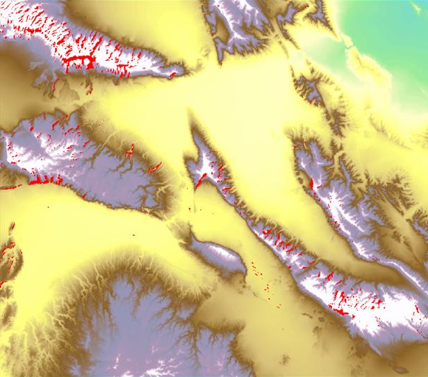
An initial assessment of the
DEM of CCB and surrounding area (Figure 3)
shows numerous small regions of null value cells (i.e. no data) for elevation
in meters, particularly on steep mountainous slopes. Null data cells were filled with interpolated
values using the following methodology recommended by Dr. Robert Tarboton,
Professor of Civil and Environmental Engineering at
- Grid cells in the “raw” DEM were converted
to points with an elevation attribute in ArcMAP Spatial Analyst; and
- Point elevation values were interpolated
back to a raster using spline interpolation feature of the ArcMAP Spatial
Analyst.
It is important to note that null elevation data cells interpolated using the spline method (shown on Figure 4) are uncertain. Dr. Daene McKinney (McKinney, 2004), a Professor at the Department of Civil Engineering at the University of Texas at Austin kindly provided extensive documentation of several ArcMAP methods fill null values (particularly for large regions of null values) in SRTM DEMs (see Appendix A). However, I chose to follow Dr. Tarboton’s approach because the number of holes in the CCB DEM were numerous but small, and I did not possess stream vectors or a 1 km2 DEM needed to apply Dr. McKinney’s methodologies.
![]()
![]()
Figure 3 – DEM (Elevation
in Meters) for CCB and Surrounding Area
Showing Null Data Cells in Red
3.3 Terrain Preprocessing
ArcHydro filled sinks in the interpolated DEM. As vector stream networks were not available
for study area, DEM reconditioning using the

![]()
![]()
Figure 4 – Interpolated DEM (Elevation in Meters) for CCB and Surrounding Area
3.4 Stream Network Generation
ArcHydro
calculated flow direction map (Figure
5) utilizing the filled DEM. Next, a
flow accumulation map (Figure 6)
was generated using the flow direction map in ArcHydro. In both figures, the beige polygon indicates
the boundaries of the Cuatro Ciénegas preserve and black lines denote
roads.
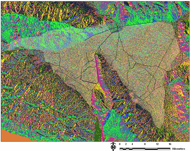
Figure 5 – Flow
Direction Map of CCB
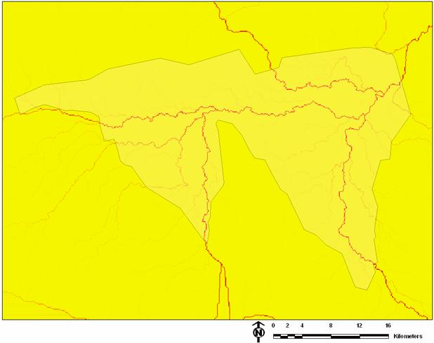
Figure 6 – Flow
Accumulation Map of CCB
Utilizing the
flow accumulation map, ArcHydro generated vector stream network for both
1 km2 and 5 km2 contributing areas (Figures 7 and 8, respectively). In each
figure, black lines indicate roads, the beige polygon outlines the Cuatro
Ciénegas Reserve, and blue lines denote streams.
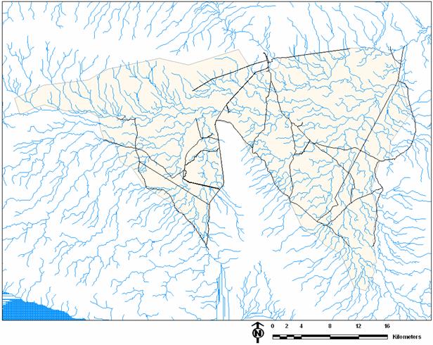
Figure 7 – Stream Network for 1 km2 Contributing Areas

Figure 8 – Stream Network for 5 km2 Contributing Areas
3.5 Hillshade Map Generation
In order to facility stream
network validation, a hillshade map was generated from the filled DEM. Stream networks generated from 1 km2
and 5 km2 contributing watersheds were superimposed on the
hillshade images (Figures 9 and 10, respectively).

Figure 9 – Hillshade Map and Stream Network for 1 km2
Contributing Areas
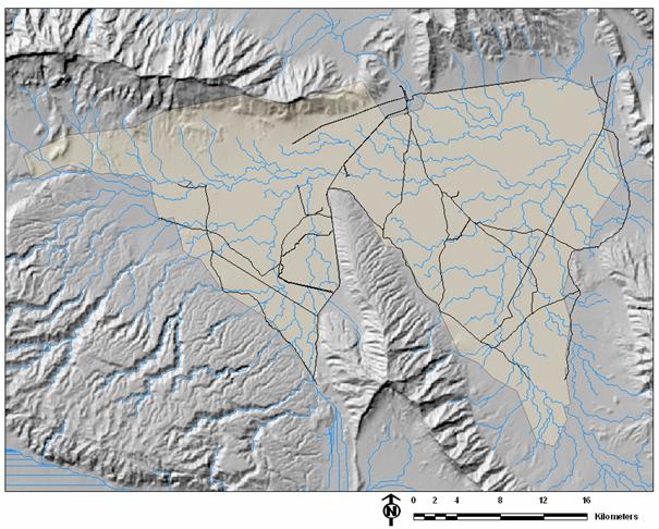
Figure 10 – Hillshade Map and Stream Network for 5 km2
Contributing Areas
3.6 Validation of Stream Network Using Hillshade Map
Visual inspection of Figures 9 and 10 indicates that streams flow down topographic lows, as
expected. However, the analysis produced
some interesting results. Even though
the basin to the southwest is internally‑draining and separated from the
CCB by a topographic high, streams were generated to connect this basin with
the lower CCB. Similarly, CCB was also
originally internally‑draining, but ArcHydro connected it with the lower
basin to the east where a canal now flows.
Finally, although a stream originally flowed from the basin to the north
into CCB, ground water withdrawals in that basin have completely captured and
dried out this stream, which no longer flows.
3.6 Validation of Stream Network Using Aerial Photos
Figure 11 shows 30 m2 aerial photos of CCB
georegistered by previous researchers and commissioned by Dr. W.L. Minckley,
a biologist who worked in CCB first in the late 1960s (as complied by Moline,
2002). The photos are superimposed on
the hillshade map and showing 1 km2 drainage basin
streams. At this scale, the streams flow
generally within drainages. However, visual
inspection of a smaller region of aerial photos (Figure 12) indicates that streams typically follow the trend
of streams, but are often slightly out of the topographic low, which may be
attributed to errors introduced when the photos were georegistered.

Figure 11 – Aerial Photos, Hillshade Map, and Stream Network for
1 km2 Contributing Areas
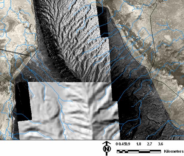
Figure 12 – Aerial Photos, Hillshade Map, and Stream Network for
1 km2 Contributing Areas Showing Stream Offset
The higher stream density of
streams generated from the 1 km2 contributing areas make them
favorable for the fracture trend analysis discussed in the following section.
4.0 FRACTURE
TREND ANALYSIS
Similarly to the Edwards aquifer recharge
zone of Central Texas, the flow of surface water runoff over limestone outcrops
generated by large mountain precipitation events may be responsible for
significant recharge to the CCB ground water system which feed discharge to the
spring system. Thus, it would be
interesting to understand the spatial distribution of fractures in the
limestone outcrops surrounding CCB. However,
the 30 m2 resolution of the aerial photos proved to be too low
to identify potential fracture zones up‑gradient of springs (which are
shown as green dots in Figure 13). As a result, field mapping of fractures by a
geologist and re‑running aerial photos at a higher resolution are
recommended to identify potential ground water recharge pathways.
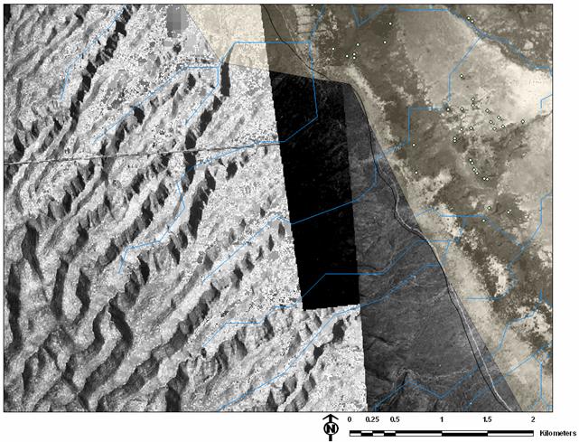
Figure 13 – Aerial Photos, Hillshade Map, Stream Network for 1 km2
Contributing Areas, and Springs (in Green)
4.1 Spatial Distribution of Springs
While the attempt to map
fractures from aerial photos was unsuccessful, an interesting discovery was
made when springs were plotted on the aerial photos. As shown in the red circle in Figure 14, a high density of
springs is found immediately down‑gradient of an approximately 6‑km
long alluvial fan developed at the foot of the limestone Sierra de


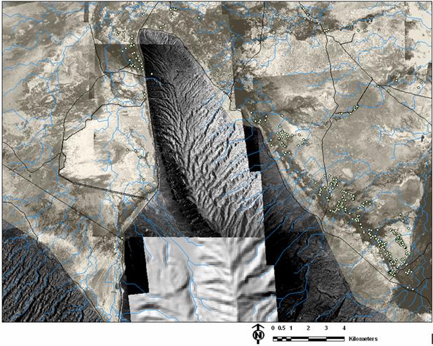
Figure 14 – Aerial Photos, Hillshade Map, Stream Network for 1 km2
Contributing Areas, and Springs (Green Dots)
5.0 CANAL
DISCHARGE OUT OF BASIN
Although CCB was originally
internally‑draining, the construction of canals in the 1900s to convey
spring water discharge out of the basin (to irrigate crops in the more fertile
valleys to the east) hydraulically linked CCB with tributaries of the
Rio Grande River (Rio Grande / Rio Bravo Basin Coalition, 2004). Figure 15
shows the spatial distribution of canals (blue lines) in CCB.
While the original intention
of this portion of the project was to populate
a geodatabase with historical canal discharge data to quantify this
component of the CCB water budget, a thorough review CCB
literature indicated that only one canal discharge measurement has been published
(Lesser y Asociados, 2001). Lesser y Asociados,
a water resources consulting firm based in Querétaro,
Mexico, measured canal discharge at the basin outlet (indicated by the green
arrow on Figure 15) at some
time in 2001 at 1,700 liters per second (which is
approximately equal to 60 CFS, or 43,000 AF/YR).
In order to generate a long-term
time series geodatabase of canal discharge, the installation of a permanent
gage at the basin outlet of the canal is recommended.

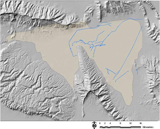
Figure 15 – Spatial Distribution of Canals
(Basin Outlet Indicated by Green Arrow)
6.0 RECOMMENDATIONS
Although
DEMs generated by the SRTM possess significant null value cells, elevation
values may be interpolated using the spline method recommended by
Dr. Tarboton in ArcMAP if null value regions are relatively small. A 1 km2 stream network
generated from a spline‑interpolated SRTM DEM of the CCB helped
understand the pre‑canal development hydrologic system and potential
ground water recharge pathways in CCB.
However, ArcHydro did not accurately model the drainage network of
internally‑draining basins or account for streams that dried up due to
regional declines in ground water level.
While remotely‑sensed images like aerial photography are useful, field visits are necessary to confirm relationships identified from remotely‑sensed images. Thus, field mapping of fractures by a geologist is recommended to identify potential ground water recharge pathways in mountainous limestone outcrops. Higher resolution aerial photography may also assist with fracture delineation. Field reconnaissance planned for January, 2005 may help understand the complex spatial relationship of springs with alluvial fans and surrounding limestone bedrock and identify potential ground water flow paths. In addition, an aerial geophysics survey utilizing gravity and magnetics may help to delineate subsurface structures such as faults or shallow bedrock features which affect the spatial distribution of springs.
The
development of a water budget for CCB is recommended in order to plan for long‑tern
sustainable development of finite CCB water resources. Water leaving the basin via discharge canals
forms a primary component of the CCB water budget. To this end, the installation of a permanent
canal discharge gage is planned for January, 2005. The recording of these discharge data in a
geodatabase is also recommended.
7.0 REFERENCES
Hendrickson, D., 2004,
Personal communication, Department of Integrative Biology, The University of
Texas at
Lesser y Asociados, 2001, Sinopsis
del estudio de evaluación hidrogeologógica e isotópica en el Valle del Hundido,
Coahuila: Comisión Nacional del Agua, Subdirección General Técnica, Gerencia de
Aguas Subterráneas.
Meyer, E.R., 1973,
Late-Quaternary paleoecology of the
Tang, C.M., Roopnarine,
P.D., 2003, Evaporites, water, and life, part I. Complex morphological variability in complex
evaportic systems: thermal spring snails from the
Tarboton, D.G., 2004,
Personal communication, Department of Civil and Environmental Engineering,
The Nature Conservancy,
2004, The Cuatro Cienegas Valley [Online]:
http://nature.org/wherewework/northamerica/mexico/work/art8626.html
[accessed on
U.S. Geological Survey,
2004, USGS Seamless Data Distribution [Online]:
http://seamless.usgs.gov/ [accessed on
APPENDIX A
Approaches to Filling Null Data Cells in an STRM DEM
Provided by Dr. Daene McKinney,
Department of Civil Engineering at
The
From: Daene [mailto:Daene@aol.com]
Sent:
To: David Maidment
Cc: brad_wolaver@yahoo.com
Subject: Re: QUESTION: Filling "no data" in DEM
Dear Mr.
Wolaver,
I have been processing the SRTM data for several parts of
the world and I have encountered this "no-data" problem. There
are several ways to fill the holes, none of which is very satisfying.
1. You can set
nodata to zero, but this does not make sense for some areas. Then you can
recondition the resulting DEM from existing streams to bring the zeros up to
surrounding values.
ArcMap: Spatial Analyst: Raster Calculator:
Con( isnull( [raster] ), 0,
[raster] )
2. If you have a
medium sized holes of nodata you can average values surrounding the nodata
using the "focalmean" function. This can take a lot of time if your
DEM is large and can require repeated use if your holes are large.
ArcMap: Spatial Analyst: Raster Calculator:
Con( isnull( [raster] ),
focalmean( [raster] , rectangle, 5, 5 ), [raster] )
You probably have to do this
several times to fill in all the holes.
Convert resulting raster back to 16-bit
unsigned integer:
ArcMap: Spatial Analyst: Raster Calculator:
Int( [raster] )
3. Another way
(especially is you have LARGE ( > 100,000 km2 areas) is to resample from the
old 1-km data and use those to fill in the holes.
Clip your basin DEM [raster], using the mask
(see below) and the larger DEM [GTOPO_30_Raster] in raster calculator
[raster]
= Mask * [GTOPO_30_Raster]
Resample GTOPO30 DEM data at 90 m and then use
Arc Toolbox: Raster: Resample (use cell size of
your DEM)
Con( isnull( [raster] ),
[resample_GTOPO_30_Raster], [raster] )
I have read a suggestion to create a TIN over the holes
using surrounding data and then interpolate on the TIN and convert that back to
the DEM, but I have not worked this out.
You
can read more about all of this at several websites:
http://www.gsd.harvard.edu/geo/manual/dem/
http://www.uweb.ucsb.edu/~nico/comp/srtm_gtopo_grid.htm
http://science.oregonstate.edu/~knochej/geo580/lab/lab6/lab6.html
http://www.arch.cam.ac.uk/comp/ac056/
http://www.css.tayloru.edu/~btoll/f04/312/res/r/Spatial.html
http://forums.avsim.net/dcboard.php?az=show_mesg&forum=124&topic_id=1459&mesg_id=1459&page=
http://www.terrainmap.com/index.html#top
http://www.vterrain.org/Implementation/Apps/VTBuilder/index.html
Please let
me know if you come up with something useful, as we are continuing to struggle
with this problem.
All the
best