Arc Hydro integrates spatial and temporal data in a hydrologic context within a GIS. In this exercise, we look at different ways of utilizing Arc Hydro’s time series format for time series display and analysis.

TimeSeries.zip contains the files used for this exercise. The data folder for this part of the exercise can be downloaded from the web site http://www.ce.utexas.edu/prof/MAIDMENT/giswr2002/ex6/timeseries.zip.

The files included in TimeSeries.zip are:

Guadalupe.mdb: An Arc Hydro geodatabase for the Guadalupe River basin

NWIS.dll: A tool used to download streamflow data from the USGS website from within ArcMap.

*Both of these files are also stored on the LRC Class server at class/maidment/giswr/timeseries.

This exercise assumes a basic working knowledge of ArcMap, the ArcGIS Hydro Data Model, and Microsoft Excel.

· To begin, unzip the contents of TimeSeries.zip to your computer.

· To start this exercise, open ArcMap, and click on the Add Data button.

· Browse to Guadalupe.mdb, and add the data in the Hydrography, Drainage, and Network feature datasets. Also add the ts_P_NEXRAD and TSType tables.

· Explore the data in ArcMap. This database contains data for the Guadalupe River basin in Texas. The database also contains more detailed data (such as Catchments) for the San Marcos River basin, which is located in the northern portion of the Guadalupe River basin. The Basin feature class represents the four USGS hydrologic cataloging units that are within the Guadalupe River basin. You can change the legend for Basin so that each of the four HUC units is labeled and has a different color, for visualization purposes.

2. Retrieving and Displaying NWIS Data

The USGS publishes real-time and historical water quantity and quality data for monitoring stations in the United States on its National Water Information System (NWIS) web site. Normally, one can retrieve the data by going to the USGS web page and navigating through various web pages. But for this exercise, we will retrieve the data automatically from within an ArcMap application, without ever having to open up a web browser. We will do this with the NWIS tool developed by the Center for Research in Water Resources (CRWR) at UT Austin.

A. Familiarizing Yourself with the Data

· For this part of the exercise, turn off all map layers except MonitoringPoint, HydroEdge, and Basin.

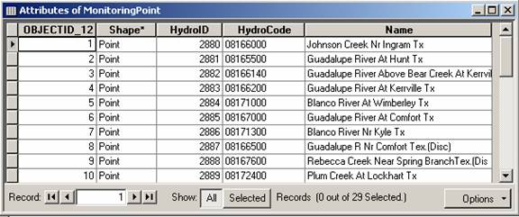
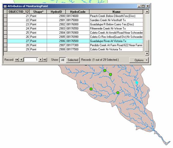
· Open the attribute table for MonitoringPoint. There are 29 MonitoringPoints in this dataset. Each MonitoringPoint represents a USGS stream gage. The 8-digit numbers in HydroCode represent USGS stream gage IDs. The NWIS tool uses the HydroCode to locate the appropriate data online for each gage.

B. Loading the NWIS tool into ArcMap

· Click ToolsàCustomize. Click the Commands tab in the Customize window, and then click Add from file.

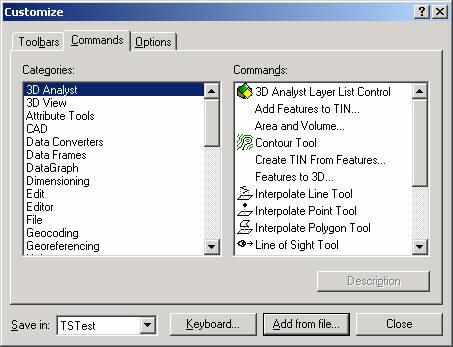
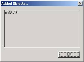
· Navigate to NWIS.dll (it is inside the zip folder for this exercise), and click Open. A window appears showing that clsNWIS was added. Click OK. Note: If you get a message saying ‘No new objects added’, then you may need to have administrator privileges to install the tool. See your network administrator for help.

· If necessary, click on ‘NWIS’ in the Categories pane of the Customize window. The Get NWIS Data command appears in the Commands pane. To add this button to ArcMap, click on ‘Get NWIS Data’ with the left mouse button. While holding down the left mouse button, drag the Get NWIS Data button next to another button in the gray area where all the commands and tools are in ArcMap. When you see the insertion cursor (looks like a capital I,) that means that tool can be placed in that location. Release the left mouse button to drop the tool in that location.

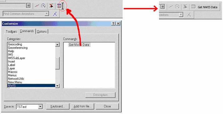
· Close the Customize window. The Get NWIS Data button is now ready for use.

C. Using the NWIS Tool

We will download daily streamflow data for the Guadalupe River at Victoria. To do this, we will select the MonitoringPoint at that location and activate the NWIS tool. The NWIS tool can download data for any number of selected gages, but we’ll just use one in the interest of time for this exercise.

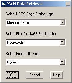
· In the attribute table for MonitoringPoint, select the record with Name = ‘Guadalupe River at Victoria TX’. This record is now selected in the table as well as the map.

· Click Get NWIS Data . In the NWIS Data Retrieval window, select MonitoringPoint as the layer, HydroCode as the USGS Site Number field, and HydroID as the Feature ID field. Then click OK.

To be turned in: What are the HydroCode and HydoID for the Guadalupe at Victoria monitoring point?

· In the NWIS Inputs window, enter 10/1/1999 as the Start Date, and 9/30/2000 as the end date, then click OK. These dates encompass the water year beginning in 1999.

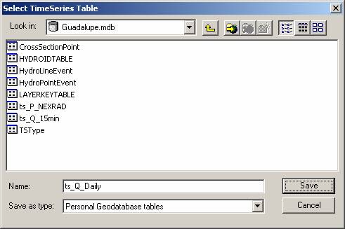
· In the Select TimeSeries Table dialog box, navigate to our Guadalupe geodatabase and type ts_Q_Daily. Then click Save. This is the table where we will store the USGS daily streamflow data.

The tool will now go to the NWIS web site and attempt to retrieve the requested time series data. A window displays the tool’s progress.

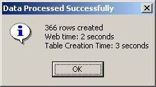
The tool ignores IDs for which no USGS gage exists. If the available data on the USGS web site isn’t sufficient to cover the entire period of record requested by the user, the tool will only retrieve the data that is available from the web site. When the tool is finished, a message box appears providing some information about the tool’s processing time. Pretty cool! You’ve just access the USGS data server in Reston, VA, at an internet address programmed into this NWIS tool, and retrieved the streamflow data without going through any html web interface at all.

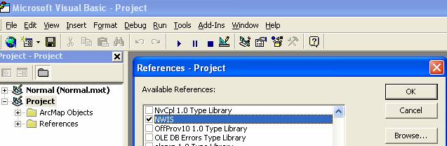
Note: If the NWIS tool produces an error, it may be due to an older version of NWIS.dll residing on your computer. You have to remove this older version of the dll for the new version works correctly. One way to check if there are old dlls is to go to Visual Basic for Applications (VBA) for ArcMap. In ArcMap, select Tools à Macros à Visual Basic Editor. In the VBA screen, choose Tools à References. Look for NWIS in the list. If it is not clicked on, then click it on:

If there is more than one, try to locate the older versions and delete them. If all else false, please email one of the authors of this exercise. A backup copy of the Guadalupe geodatabase with the time series data added is available at http://www.ce.utexas.edu/prof/maidment/giswr2003/ex6/GuadalupeSolution.Zip

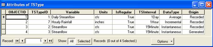
If your time series table does not show TsTypeID = 1 (e.g. it has a value of 0 for this field), using the Table Calculator, set TsTypeID = 1 for the daily streamflow data you’ve just downloaded. The TSTypeID identifies categories of time series data, e.g. rainfall data might have a TSTypeID of 7, while daily streamflow data might have a TSTypeID of 1. The TSTypeID will link each time series record to a row in the TSType table, which provides descriptive information about categories of time series data.

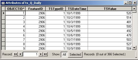
In the ArcMap open the TSType and ts_Q_Daily tables and inspect the data. Note how the TSType table describes the time series data as Daily Streamflow, in units of cfs, at regular intervals, etc. We’ll use the type 7 for Nexrad data later.

You can use the Statistics tools in ArcGIS table display to define the statistics of a dataset. Right click on the field you want to summarize and select the S Statistics option.

You’ve now loaded one water year of daily streamflow data into a table in ArcGIS. In the next part of the exercise, we will use Excel’s capabilities to create a graph of time series data for the Guadalupe River at Victoria.

To be turned in: What is are the mean, minimum and maximum daily flows (cfs) for the Guadalupe River at Victoria in the 1999-2000 water year (October 1999 – September 2000) ? What is the volume of water (ft³) which passes through the gaging station in this year?

D. Displaying Time Series in Excel

While ArcGIS is a powerful tool for displaying spatial data, the graphing capabilities of Excel provide a useful tool for displaying certain time series data. Because ArcGIS uses a relational database format to store its data, these data can be imported into Excel. In this portion of the exercise, we will import daily streamflow data for the Guadalupe River at Victoria and plot a graph.

· Save the ArcMap document as Guadalupe.mxd, and then close ArcMap.

· Open Microsoft Excel.

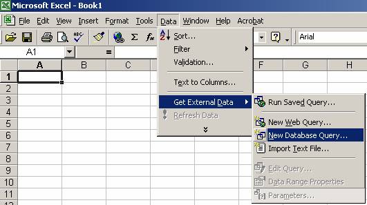
· Click DataàImport External DataàNew Database Query…

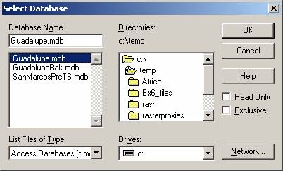
· In the Choose Data Source dialog box, click MS Access Database* and then click OK.

· Navigate to Guadalupe.mdb and click Open.

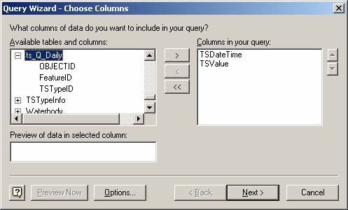
· In the Choose Columns window, locate the ts_Q_Daily table, and expand its entry by clicking the + sign next to it. This displays the fields in ts_Q_Daily.

· To make the plot, we will use the TSDateTime and TSValue fields. Highlight TSDateTime by clicking on it, and then click the > button to move that field to the Columns in your query: text box.

· Follow the same steps to place TSValue in the window.

· Click Next.

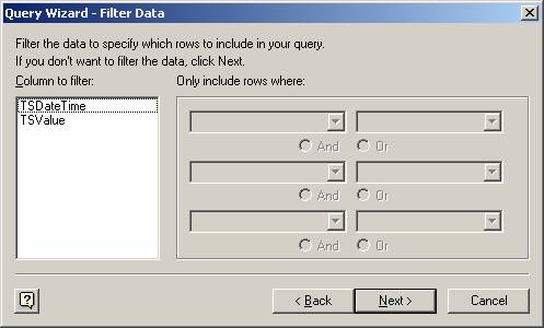
· We will not filter the data. In the Filter Data window, just click Next to continue.

· We will sort the data in chronological order. Choose TSDateTime in the Sort by combo box, and make sure Ascending is selected in the options on the right. Then click Next.

· In the next window, choose Return Data to Microsoft Excel option, and then click Finish.

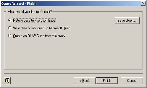
· The next window prompts you for the location where the data will be placed. Cell A1 in the existing worksheet is fine. Click OK.

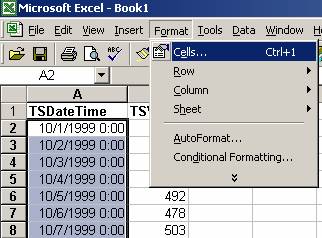
The data are loaded into Excel. Date fields in ArcGIS store date information down to the millisecond, although date values are displayed according to the precision of the value. Thus, even though the data in ts_Q_Daily represent daily records, Excel detects a higher precision, hence the MM/DD/YYYY 0:00 format in the TSDateTime field.

· To change the TSDateTime field to display daily precision, highlight all of the values in that field, and then click FormatàCells.

· Choose Date as the Category, and 3/14/98 as the type. Then click OK.

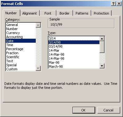
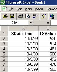
The data are now displayed with daily precision.

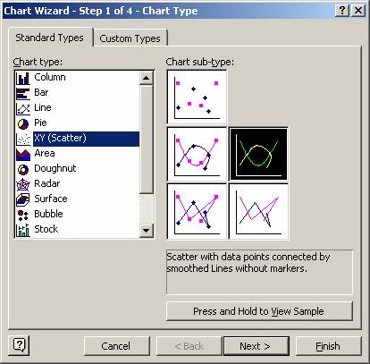
· To make the plot, select all of the data, and then click the Chart Wizard button.

· In Step 1 of the Chart Wizard, choose XY (Scatter) as the chart type and select the graph option for just lines (the default is for just points):

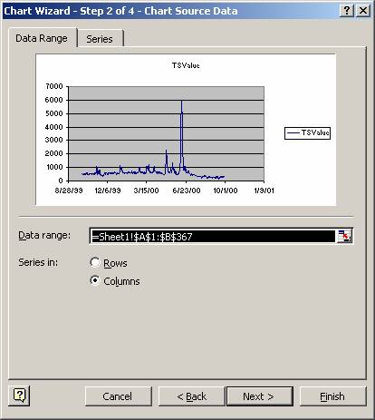
· In Step 2, make sure Columns is selected as the Series in: option. Click Next.

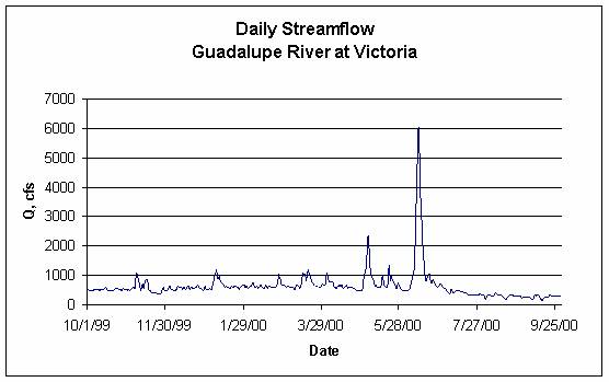
· In the next two windows, you can customize the look of the plot as you see fit. The finished result may look something like this.

· You may now save your results and close Excel.

Congratulations! You have loaded daily streamflow data from the Internet into ArcGIS, and created a plot of the data in Excel. You are a multi-application master!

To be turned in: Make a layout showing the basin, streamflow station, and the excel plot of daily streamflow data (make your own design).

3. Viewing Time Series in a GIS

Graphs of time series data for a single feature can be plotted quite elegantly in Excel, but when viewing time series for multiple features simultaneously, the GIS may be the better tool for the job. ESRI has developed an extension for ArcMap called the Tracking Analyst for viewing temporally varing spatial objects. This exercise will show how to use the Tracking Analyst extention to visualize a storm event over the San Marcos River Basin.

The Tracking Analyst is quite flexible in the format of data required and the options for symbolizing and rendering the spatial features according to the magnitude of their time series value for a given time-stamp. The required information is a shape, a date, and a value (i.e. where, what, and when) that can be stored in one feature class or one feature class and one associated table. This flexibility allows the Tracking Analyst to display features that move and/or change shape through time in addition to features that have time-indexed attribute values. Below is a list of possible scenarios for features changing through space and over time and a hydrologic example of each.

Stationary features with static shape (e.g. a stream flow gage)
Stationary features with dynamic shape (e.g. an inundated river)
Moving features with static shape (e.g. following a control volume)
Moving features with dynamic shape (e.g. a storm event)

Let’s get started with using Tracking Analyst to display rainfall data for NEXRAD Next Generation Radar (a Doppler Radar) cells over the San Marcos River Basin.

A. Familiarizing Yourself with the Data

· If necessary, open Guadalupe.mxd.

· For this part of the exercise, turn off all map layers except HydroResponseUnit and Basin. HydroResponseUnit represents the NEXRAD rainfall cells for the San Marcos River basin. Each cell has an hourly rainfall time series associated with it over the period 10/12/2001 11:00 pm to 10/13/2001 2:00 pm.

· Turn off the Basin map layer.

· Open the ts_P_NEXRAD table. This table contains the hourly rainfall data for the NEXRAD cells. Each record is linked to a particular cell through the FeatureIDàHydroID association. Close the table.

B. Loading the Tracking Analyst Extension into ArcMap

· If the Tracking Analyst toolbar is not present on the ArcMap user interface, click ViewàToolbars, and then select Tracking Analyst. This displays the Tracking Analyst toolbar (shown below).

· Check to make sure the Tracking Analyst extension is selected (if not, the buttons on the Tracking Analyst will be disabled). Click ToolsàExtensions. Click on the box next the “Tracking Analyst” if it is not already checked.

C. Creating a Temporal Layer

· We will now create a Temporal Layer using the HydroResponseUnit feature class and the TimeSeries (ts_P_NEXRAD) table. Click the button on the Tracking Analyst toolbar. Select the second option for the first question (What data do you want to add into your map as a temporal layer), browse to the input feature class (HydroResponseUnit from the Hydrography Feature Dataset) and then to the input table (ts_P_NEXRAD). Finally, select TSDateTime from the input table as the date/time field. The form should look like what’s pictured below. Click Next.

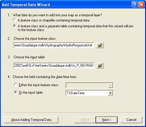
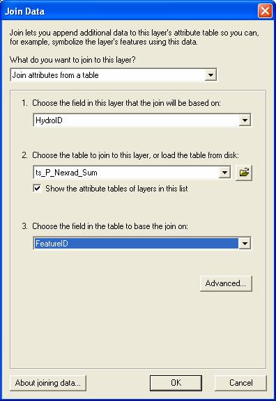
· Choose HydroID as the join field in the input feature class and FeatureID as the join field in the input table. This will provide the link between features in the feature class and their associated time series records. Click Finish. It should only take a few seconds for ArcMap to generate the temporal layer named ts_P_NEXRAD & HydroResponseUnit. This new layer is simply the HydroResponseUnit featureclass joined to ts_P_NEXRAD time series table. Open up the layer’s attribute table to take a look.

D. Setting the Temporal Layer’s Symbology and Visualizing the Storm Event

If you open the attribute table for the new temporal layer ts_P_NEXRAD & HydroResponseUnit, you’ll see a table with 4,768 features, each one representing one time series record for one feature. We’ll now symbolize this layer to show the storms movement over the San Marcos River Basin.

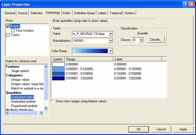
· Right-click on the ts_P_NEXRAD & HydroResponseUnit layer and select the properties/symbology tab.

In the top left corner in the Show box there are three options. The Events option controls how the features are symbolized for each time step. The Time Window option allows you to change the event symbology as time progresses. The Tracks option can be used to connect features as they move through time (i.e. to show the path of an airplane as it moves). For this exercise, we’ll only use the Events option, but if you’re interested, play around with the Time Window to understand how it works.

· Make sure the Events option is highlighted in the Show box. In the Drawn As box, select Graduated colors under the Quantities heading. For the Fields value, select ts_P_NEXRAD.TSValue as the value (see figure below). Click the Classify button and chose to classify the values into 4 Quantiles. Finally, make the first quantile (zero values) hollow and the others three increasing shades of blue.

· Now go to the Temporal tab. Select to display only the most current events in the Window. This will insure that Tracking Analyst only renders the rainfall for the current TSDateTime and not past TSDateTimes.

You have now symbolized the temporal layer and are ready to animate the rainfall over time.

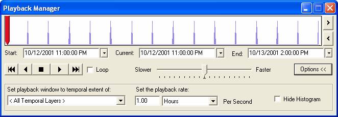
· Press the button on the Tracking Analyst toolbar. This will launch the Playback Manager (shown below). Click Options and set the playback rate to 1 hour. You can press the play button to start the animation, or just move the red bar to the right. Try both approaches.

Tracking Analyst can also be used to make a movie of the NEXRAD data over the Hydro Response Units.

The movie can then be put into PowerPoint or on the web and act as a power visualization tool.

· On the Tracking Analyst toolbar, press Tracking Analyst à Animation Tool. Keep the Date Range as is, choose to create a frame every hour, keep the animation format and the frame size the same, and finally set the path to your working directory and name the file GuadalupeNEXRAD.avi. Press Generate and when the tool is finished, navigate to it with Windows Explorer and play the movie (you will need software that can play video files, such as Windows Media Player).

To be turned it: In the same way you used Excel to plot streamflow time series for one gage, use Excel to plot the rainfall for one or more of the cells in the HydroResponseUnit. Make a layout showing the HydroResponseUnits and the Excel plot clearly indicating what cell you are plotting time series for. Here’s an example:

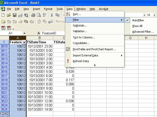
You can create these graphs in Excel using the same procedure as described earlier for the streamflow data graph. In this instance, you want to use Data/Get (or Import) External Data in Excel to get the ts_P_Nexrad table in the Guadalupe.mdb file, select the FeatureID, TSDateTime and TSValue fields for import into Excel, sort by FeatureID, and then sort by TSDateTime to get the following display in Excel. The data display shown has records only for FeatureID 10612. This is done in Excel by highlighting the FeatureID column, and using Data/Filter/AutoFilter which then enables data for any individual FeatureID value to be displayed.

While having the rainfall data geospatially reference by the Hydrologic Response Units (or the NEXRAD cells) is useful, potentially more useful is having the data geospatially referenced by the catchments. This is a first step in using the rainfall to estimate streamflow. The next part of this exercise, therefore, is to transfer the rainfall from the HydroResponseUnits to the catchments

E. Transferring Rainfall from HydroResponseUnits to Catchments

This is a somewhat painstaking process, so the methodology will be presented here for your knowledge, but you will not be expected to reproduce the process. Instead, you’ll just use the end product: TimeSeries records for the catchments.

The steps in transferring the rainfall from the HydroResponseUnits to the Catchments are:

1. Select data with a unique TSDateTime from the TSTimeSeries table.

2. Join the selected set of time series with the HydroResponseUnits

3. Convert the HydroResponseUnits from features to a raster with the TSValue as the attribute.

4. Perform zonal statistics on the raster using the Catchments.

5. Add a field to the zonal statistics table and populate the field with the TSDateTime used.

6. Load this data into the TSTimeSeries table as TSType 7 and FeatureID = Catchments HydroID.

7. Repeat steps 1-6 for all unique TSDateTimes.

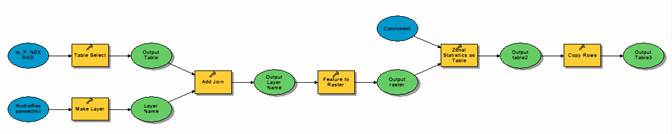
Model builder, avaibale in ArcGIS 9.0, is ideal for automating this process. Below is an example of how one step might be accomplished in Model Builder. This model could then be executed for all TSDateTime values using a script.

As mentioned before, the process of transferring data from the HydroResponseUnits to the Catchments has already been completed and you are not expected to reproduce the results. Instead, just use the results stored in the ts_P_NEXRAD table.

F. Visualizing the Storm Event on the Catchments

We will now create a second temporal layer, this one a combination of the catchments and the ts_P_NEXRAD TimeSeries table. This second temporal layer will show the storm event spatially aggregated by the catchments instead of the HydroResponseUnits.

· Click the button on the Tracking Analyst toolbar. Select the second option for the first question (What data do you want to add into your map as a temporal layer), browse to the input feature class (Catchment) and then to the input table (ts_P_NEXRAD). Select TSDateTime from the input table as the date/time field and click Next.

· Right-click on the ts_P_NEXRAD & Catchment layer and select the symbology tab.

The Tracking Analyst allows you to visualize the storms path over the basin. Pretty cool stuff! Of course you can use Tracking Analyst for other visualizations pertinent to water resources engineering. In the first part of this exercise we looked at stream flow at one gaging station. We could, rather easily, download streamflow data for all of the gages in the Guadalupe Basin and use the Tracking Analyst to visualize how stream flow is changing over time. This, together with the NEXRAD rainfall data, is a powerful method for visualizing how a basin responds to a storm event.

G. Performing Rainfall Analyses with the Results

With the standard Arc Hydro tools, we can perform some useful analyses with our NEXRAD time series data. In this portion of the exercise, we will determine the total volume of rainfall that fell each catchment and then we will accumulate this incremental rainfall downstream to find the total volume of rainfall that fell on or above each catchment. To do this, we’ll use a Microsoft Access query and the Arc Hydro Accumulate tool.

Preparing the Data for the Accumulate Tool

We’ll use Access to sum all time series values for each FeatureID to calculate the total depth of rainfall for each catchment. Access is a very powerful tool to know when working with geodatabases. It is often the best tool for the job, especially for non-spatial queries like this.

Save the map document (name it TimeSeries.mxd if you’d like) and close ArcMap.
Start Microsoft Access . Access is the relational database system that is part of the MS Office package, so you start it from the Start button in Windows just as if you were using Powerpoint.
Browse to and then open the Guadalupe.mdb file.

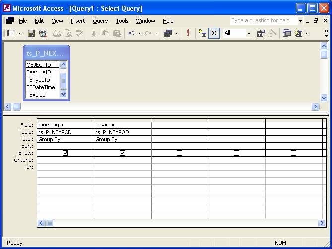
We are going to build a query and then use that query to produce a new table that has the HydroResponseUnit and Catchment HydroIDs in one field, and the sum of all TSValues in the second field.

· On the left-hand side of the active window, highlight Queries under the Objects heading.

· Double-click Create query in Design view.

· In the Show Table window, highlight ts_P_NEXRAD and click Add.

· Close the Show Table window

· Click and drag FeaureID down to the fields (see below).

· Do the same for TSValue

· On main menu bar Click View àTotals. This adds a new row to the fields called Total. (This can also be done by right clicking on the field and selecting the S Totals option)

· Change the Total row from Group by to Sum for TSValue. This will sum up the rainfall in TSValue for each FeatureID. Use the little right arrow at the top right of the field to do this.

Total Row Added

Change to Sum

Click and drag FeatureID and TSValue down to Fields

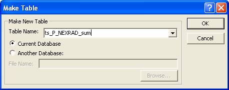
· Click the down arrow next to the button to change the Query Type to a Make-Table Query.

· Name the table ts_P_NEXRAD_sum and press OK.

· Run the Query by using the Run ! button. This will create a new table based on your query and save that table in the Guadalupe database.

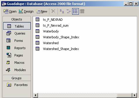
You can check that you’ve created the new table by going back to the main screen, clicking on Tables, and scrolling to the right hand side of the display where you’ll see ts_P_Nexrad_sum.

That’s it for Access. Now let’s go back to ArcMap.

· Close Access (save the query and the database) and open ArcMap. Open the map document you were previously working on.

If you did not succeed in doing the part in Access and want to continue with the exercise, you can find a solution file at http://www.ce.utexas.edu/prof/maidment/giswr2003/ex6/GuadalupeSolution.Zip

that has the required ts_P_Nexrad_Sum table in it.

The next step is to transfer the consolidated rainfall values from the table we created to the Catchment feature class.

· Right-click on the Catchment Layer and open its attribute table

· Create a new field call incRainfall (type double). (Optionsà Add Field)

· Close the attribute table.

· Right-click on the Catchment Layer, select Joins and Relates and then Join.

· Join the Catchment Layer with the table we just created (HydroID = FeatureID) as shown below. Press OK.

· Open the attribute table for the catchment layer.

· Right-click on the incRainall and choose to calculate values (if this option is not available, start an editing secession as discussed below).

· Let the calculated values = the SumOfTSValues in the table created by the Access query.

If the Add Field option is not active, then you might be in an edit session. You cannot add fields if you are in an edit session. If necessary, Click EditoràStop Editing, and then try adding the field. If you still cannot add a field, save your Map file, close ArcMap, go to the folder where your geodatabase is stored and delete a small 1KB file that is called Microsoft Access Record-Locking Information, open ArcMap back up again, and proceed.

You now have the total incremental rainfall for each catchment summed over the duration of the storm event. Before accumulating the rainfall downstream, we must first calculate the total volume of rain that fell on each catchment (i.e. change the units of the rainfall from Length to Volume).

Remove the Join between Catchment and ts_P_Nexrad_Sum:

These catchments were processed from raster data using the Arc Hydro tools. Thus, the NextDownID attribute is populated. This ID points to the HydroID of the next downstream Catchment. We can use this attribute to accumulate rainfall totals from upstream catchments to downstream catchments. But first we must add a field to store the total rainfall.

· In the attribute table for Catchment, click OptionsàAdd Field. Create a field called incRainVolume of type Double.

· Calculate this new field with the expression:

[Catchment.incRainfall] * [Catchment.AreaSqKm] *25400

This gives us an estimate of the total volume of rain that fell on each catchment. The rainfall values are in inches and the catchment areas are in square km, so the 25400 conversion factor is the result of (10⁶ m²/km²) * (1m /39.37 inches), so that the resulting volumes appear in cubic meters. The results should look like this…

Running the Accumulate Tool

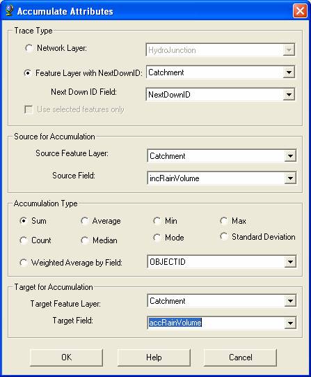
· We’ll now accumulate this incremental volume of rain water for each catchment downstream to understand how water accumulates through the basin. In the attribute table for Catchment, click OptionsàAdd Field. Create a field called accRainVolume of type Double.

· On the Arc Hydro toolbar, click Attribute ToolsàAccumulate.

· Click Feature Layer with NextDownID as the Trace Type.

· Choose Catchment as the Feature Layer with NextDownID.

· Choose NextDownID as the Next Down ID Field.

· Make sure that Use selected features only is not checked.

· Choose Catchment as the Source Feature Layer.

· Choose incRainVolume as the Source Field.

· Click Sum as the Accumulation Type.

· Don’t use a weighted average

· Choose Catchment as the Target Feature Layer.

· Choose accRainVolume as the Target Field.

· Click OK.

The Accumulate tool uses the NextDownID—HydroID association to determine which catchments are upstream of the outlet catchment. It then sums the rainfall totals (from the incRainVolume field) from those catchments and adds it to the rainfall of the outlet catchment.

· When the tool is finished (it will take a few minutes). The accumulated volume of rainfall should look like this…

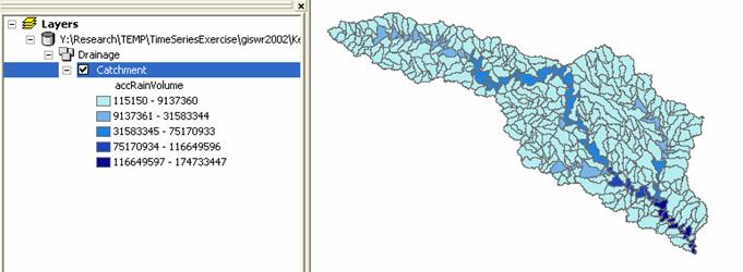
Notice the accumulation of rain along the Guadalupe River?

To be turned in: What is the average depth of rainfall during this storm over the whole San Marcos basin covered by these catchments? Express the result in mm of rainfall.

Congratulations! You have produced some cool time series animations in a GIS and used NEXRAD data to determine the amount of rainfall each San Marcos catchment received during a storm. You have also determined the accumulated volume of rain and its flow path for the San Marcos River basin for a given storm. Pretty cool stuff!

Summary of items to be turned in:

(1) What are the HydroCode and HydoID for the Guadalupe at Victoria monitoring point?

(2) What is are the mean, minimum and maximum daily flows (cfs) for the Guadalupe River at Victoria in the 1999-2000 water year (October 1999 – September 2000) ? What is the volume of water (ft³) which passes through the gaging station in this year?

(3) Make a layout showing the basin, streamflow station, and the excel plot of daily streamflow data (make your own design).

(4) In the same way you used Excel to plot streamflow time series for one gage, use Excel to plot the rainfall for one or more of the cells in the HydroResponseUnit. Make a layout showing the HydroResponseUnits and the Excel plot clearly indicating what cell you are plotting time series for.

(5) What is the average depth of rainfall during this storm over the whole San Marcos basin covered by these catchments? Express the result in mm of rainfall.