Mohamed Rachid El Meslouhi
Direction Generale de l'Hydraulique
Rabat, Morocco
November 1996
The goals of this exercise are to give you an understanding of how Arc View can be applied to study river basin management using the Souss Basin in Morocco as a case study example. The exercise consists of these parts:
The simulation of the Souss basin also needs to account for the presence of three large dams in the basin and for exchange of water between the surface and shallow groundwater systems. Work on these aspects of the model is continuing. Without these items included in the surface water simulation, the results are rather approximate. But the intent here is to document how to build a model. Exercise 2 shows in a more fully developed way how to run a model which is already constructed.
The watershed delineation portion of this exercise requires ArcView 3.0 with the Spatial Analyst and Hydro extensions. The remainder of the exercise requires ArcView GIS, version 2.1 or later. ArcView is developed by the Environmental Systems Research Institute (ESRI), Redlands, California.
The files required for this exercise are in the directory rivers\ex1\gisfiles\ on the CD-ROM. Create a new workspace, say souss and open a MS-DOS command prompt. Copy the files from the CD into the workspace by typing the following command at the DOS command prompt. (Substitute your CD drive for D in the command if the CD drive on your computer is not D).
xcopy D:\rivers\ex1\gisfiles C:\souss\gisfiles /e
where the D drive is the directory containing the CD-ROM and C drive is the drive containing the newly created souss directory. Copying files in this manner ensures that the permissions on the files are changed from the Read Only (automatically assigned to files on the CD-ROM) to Read-Write. If the file manager or the copy command is used to copy these files, the permissions on the individual files will need to be changed to Read-Write.
File(s) for Part 1
The grids, nwa_2 and sodempl, are located in the directory rivers\ex1\gisfiles\grids
File(s) for Parts 2 - 4
The Souss Basin has an area of approximately 20,000 sq. Kilometers and is located at the Southern end of the Atlas Mountains. It was selected for this study because it contains a central valley having a large shallow groundwater basin fed by drainage from the overlying Souss River and from the Atlas Mountains. This valley is pumped heavily to support irrigated agriculture, especially citrus fruit production, and water levels are declining in the aquifer. Several plans have been put forward to replenish the groundwater by artificial recharge. Some of these plans include providing using small spreading berms on the Souss river and building a canal to divert part of the Souss river flow to an area of the valley floor in which it can be used for groundwater replenishment. Another plan calls for reduced reliance on ground water. This could be done by building more reservoirs in the mountains to create additional surface water supplies. All these alternatives involve interactions between groundwater and surface water. It is intended that GIS-based models should provide a basis for studying project alternatives in the effort to define a feasible approach to alleviating water shortages in the basin.
Start ArcView 3.0 and open the project called delin.apr . The pointers for the grids and value attribute tables (.vat) may need to be updated. If this is the case, a window will come up asking you to point out the location of the files. The grids, nwa_2 and sodempl, are stored in the river\ex1\grids directory while the .vat files are stored in the river\ex1\grids\info directory. Browse through the directories to locate the file and correct the pointers by double clicking on file.
You will notice that the menu options for "Analysis" and "Hydro" appear in the View Menu Bar. These additional options are part of the Spatial Analyst and Hydrologic Modeling extensions. Extensions contain customized buttons, tools, menus and their associated Avenue Scripts and are added to the basic ArcView program to perform special functions. To see how these Extensions were added to this project, make the project menu active and look at the menu item File/Extensions . You will see a check mark next to the Hydrologic Modeling and Spatial Analyst extensions. These two extension are supplied by ESRI. The menu "Hydro" has been modified from its original form for this exercise by installing an extra tool and a button in View menu bar.
To take a look at the area you will be working with, open the View BigDem. You will see a digital elevation model of northwest Africa with a box outlining the area of the DEM that was used to analyze the Souss Basin. This DEM was prepared by Michael Hutchinson and his co-workers at Australian National University and has a cell size of 3'. The high Atlas Mountains lie to the North of the Basin while the central plain contains the Souss River, which flows into the Souss River at the Atlantic Ocean at Agadir. The elevations in this region range from 0 to 4500 m, here shaded in 500m increments. The region of the Souss Basin is shown in the small box, where the Atlas mountain range reaches the Atlantic coast.
You can use the ![]() tool
in ArcView to zoom in on the Souss region and the
tool
in ArcView to zoom in on the Souss region and the ![]() tool to examine the elevations on the grid. You'll see that the elevations
range from 0 at the coast to a little over 4000 m at the highest cell.
If you highlight the DEM theme and select Theme/Properties, you
will see that the cell size is 0.05 degrees, or 0.05 x 60 = 3 minutes.
This corresponds to a little more than 5 km on the ground. This particular
grid was developed for purposes of climatic interpolation, and 3' cells
are appropriate for describing average climatic conditions.
tool to examine the elevations on the grid. You'll see that the elevations
range from 0 at the coast to a little over 4000 m at the highest cell.
If you highlight the DEM theme and select Theme/Properties, you
will see that the cell size is 0.05 degrees, or 0.05 x 60 = 3 minutes.
This corresponds to a little more than 5 km on the ground. This particular
grid was developed for purposes of climatic interpolation, and 3' cells
are appropriate for describing average climatic conditions.
Close this view and open the View delin. You will see the clipped portion of the DEM that we are actually going to use for watershed and stream network delineation of the Souss basin. This DEM originally had a cell size of 30" and was developed by Sue Jenson and her co-workers of the US Geological Survey in Sioux Falls, South Dakota from the Digital Chart of the World. This grid is available for all of Africa on Internet, and similar DEMs are also available on Internet from the USGS for the other major continents. The DEM shown here was clipped from the Africa continental DEM and projected into a Lambert Conformal Conic projection which is a standard for this region of Morocco.
The Theme name for this grid is sodempl. You can determine some
information about this grid by making it active and selecting Theme
/ Properties . You will see that the cell size for this DEM is 1000
m and the number of cells in the grid is 206 by 239 for a total of 49,234
cells. Click OK to close this window. You will now use the Hydrologic modeling
extension, Hydro, to process this digital elevation model.
Make sure that sodempl is the active Theme and then select from
the Menu options the menu item Hydro / Flowdirection . A new grid
called Flow Direction is computed using the 8-direction pour point
method and added to your View. Take a look at this grid by placing a check
mark next to the Theme name. Each cell in this grid has the value 1, 2,
4, 8, 16, 32, 64, or 128 indicating that the flow direction is in the east,
southeast, south, southwest, west, northwest, north, or northeast directions
respectively.
You can use the Hydro extension to calculate a histogram showing the number
of cells in the grid flowing in each direction by making the Flow Direction
theme active and clicking on ![]() in the View Menu bar. If you use the
in the View Menu bar. If you use the ![]() tool you can click on the bars of the histogram and see the "count"
or number of cells which flow in this direction. The principal flow directions
are to the South, West and Southwest, reflecting the drainage of water
south out of the Atlas mountains and then West to the Atlantic Ocean. There
is also a significant flow coming North from the lower mountains forming
the Southern boundary of the basin. Close this histogram window in the
View.
tool you can click on the bars of the histogram and see the "count"
or number of cells which flow in this direction. The principal flow directions
are to the South, West and Southwest, reflecting the drainage of water
south out of the Atlas mountains and then West to the Atlantic Ocean. There
is also a significant flow coming North from the lower mountains forming
the Southern boundary of the basin. Close this histogram window in the
View.
Remove the check mark next to the flow direction grid so that you can
see the DEM again. A script is available that traces the flow path of water
from any cell in the DEM to the edge of the DEM. To activate this script,
click on ![]() and then click
on any location in "sodempl." Click on as many points as you
wish. The lines that have been drawn are graphic objects in ArcView. To
remove these graphics, select Edit / Select All Graphics and then
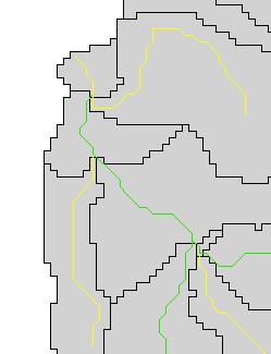
select Edit / Delete Graphics . The three upper paths shown here
all drain to the Souss river, while the fourth path to the South flow through
a separate outlet to the ocean, included in the study because its drainage
area also overlies the Souss aquifer.
and then click
on any location in "sodempl." Click on as many points as you
wish. The lines that have been drawn are graphic objects in ArcView. To
remove these graphics, select Edit / Select All Graphics and then
select Edit / Delete Graphics . The three upper paths shown here
all drain to the Souss river, while the fourth path to the South flow through
a separate outlet to the ocean, included in the study because its drainage
area also overlies the Souss aquifer.
To identify the drainage network, again make the Flow Direction Theme
active and then select Hydro / Flow Accumulation from the View menu
bar. This causes ArcView to run the Flow Accumulation function, which counts
the number upstream cells of each cell in the grid, and places the result
in new grid. If you place a check mark next to the Flow Accumulation Theme,
you will see that major drainage paths are displayed in darker colors.
The numbers in the legend bar specify the number of upstream cells whose
drainage passes through the given cell. Since each cell in this grid has
size 1 km, these numbers are the same as the upstream drainage area of
each cell in sq. km. The cells in the white area in the illustration below
have upstream drainage area less than 70 sq. km. If you zoom in to the
region of the two watershed outlets in the study area, you can use the
![]() tool to determine the
flow accumulation of each outlet. The values are 17,989 sq. km and 5152
sq. km, respectively, so the study region has a total drainage area of
23,140 sq. km.
tool to determine the
flow accumulation of each outlet. The values are 17,989 sq. km and 5152
sq. km, respectively, so the study region has a total drainage area of
23,140 sq. km.

A drainage network is defined in the next step by creating a new grid
whose cells are classified in those with value 0 or 1, where 1 means that
the cell is on a stream and has a Flow Accumulation value greater than
a specified threshold number (or drainage area) and all other cells have
the value 0 so they constitute the "landscape" or off-stream
cells. This is carried out by highlighting the Flow Accumulation grid and
then selecting Analysis / Map Query from the View Menu bar, using
the editor window to ([flow accumulation] > 500 ) and then hitting the
Evaluate button. By repeating this exercise for different threshold values,
you can get a sense for stream networks of different degrees of detail.
The resulting stream network can be overlaid on the DEM grid:
To delineate watersheds, select the menu item Hydro / Delineate Watersheds
. Make sure that the Theme names specified are correct and click OK
at the first message box.
At the second message box, you are allowed to specify the delineation threshold
for creating a set of watersheds. Leave the prefix at "xx" and
the threshold at 100 cells and click OK. The prefix is a two letter identifier
for this particular watershed delineation. If you want to repeat the exercise
for an alternative threshold stream drainage area, you must choose a different
prefix identifier for the new grids thus created.
Click OK when the program finishes.
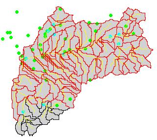
This program creates a classified stream network with 1's in the streams and 0's elsewhere (xxst) and a grid of delineated watersheds (xxshd). The watershed delineation program uses the logic that a stream is begun whenever the cells have a drainage area greater than the threshold of 100 cells (or 100 sq. km in this case), and a watershed is delineated for each stream link with its outlet cell at the stream junction where this link discharges its water into the next downstream link. Each watershed has a unique grid-code. It is much easier to view the watersheds if they are converted to polygon features. To convert the watersheds to polygon features, click on the C button.
Place a check mark next to "xxshdc" to see the watersheds
you have delineated. It may be easier to see the results of the next step
if you change the legend for these watersheds to white.
To display the delineated streams on top of these watersheds, drag the
Theme xxst to the top of the Legend Bar. Here is the result for
the 100 cell flow accumulation. It is complicated! Simpler networks can
be created by increasing threshold accumulation.
Now, we will switch to the part of the exercise that can be executed with either ArcView 2.1 or ArcView 3.0. The inputs to this exercise include the watershed and stream network computed in the previous part of the exercise.
The project called hydro97.apr contains many scripts that are used to simulate surface water flow. To set up the surface water simulation model for the Souss Basin, open the project hydro97.apr. Open a new View and add the arc coverage soriver, the polygon and arc coverages for sobasin, and the point coverages rainst and hydrost.
The point, arc and polygon coverages of the watershed, sobasin are stored in a folder. To add both the polygon and arc coverages in this menu, click on the folder next to sobasin and the select the themes from the resulting list. Place a check mark in the little box next to each theme in the view legend, to make the themes visible. Remember to keep point themes on top of line themes, and line themes on top of polygon themes in the view legend. Rainst contains stations where rainfall records are available and hydrost is a map of runoff stations.
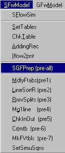
Run the one step preprocessing procedure by selecting SGFPrep (pre-all)
from under the SFlwModel menu of the View Menu Bar. By selecting
SGFPrep (pre-all), you are essentially selecting the eight processes
in the tool bar simultaneously.
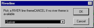
A series of dialogs are initiated to specify the required coverages and the number of time steps to be used in the optimization procedure. Preprocessing the coverages in this manner results in a transfer of process control to the program. Any errors encountered during the run will be ignored and the errors will be propagated. Errors typical arise from reusing coverages that have previously been modified for use in another model or operating system. Hence, if an error message is encountered during the run, stop the process and restart processing using coverages imported from the export (*.e00) format. The first dialog box will prompt you to for a river theme. Select Soriver.
The next dialog will ask for a polygon theme. Select Sobasin. The final prompt will ask for a basin-boundary theme. Select Sobasin.
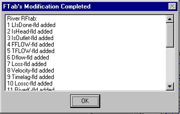
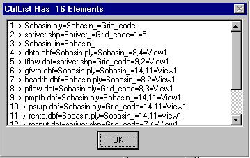
ArcView will then run the program, and a list of modifications similar to the one below will appear. You must click OK for the program to continue.
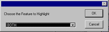
You will then be prompted to choose a feature to highlight . Select both to highlight both head and outlet sections.
You will then be prompted to confirm whether or not to Hightlight Exits. Select Yes. The final prompt will again seek confirmation of the feature to be highlighted; Highlight Exit . Again, select Yes.
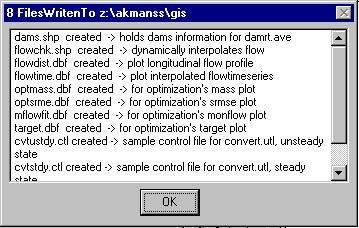
As ArcView processes the information, you will be prompted to save soriver.shp and sfdbfs.ctl in your directory. The following box will appear letting you know that ArcView is still processing. Simply click OK to continue.
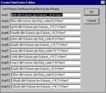
You will again be prompted to choose a feature to highlight; select both. The next dialog box presents a list of time series tables to be created. Click OK to use the default settings.
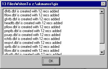
The next step will be save your files to the proper directory. You must then choose a number of records to evaluate. For this example we chose a monthly record, hence 12 periods. ArcView will then create and add 12 new tables to your project.
ArcView will also create new shapefiles. Click OK to continue.
You will then be asked whether or not you want to keep the graphics.
Choose No.
ArcView then creates a 'mold' for flowchk and dams. However,
as this point these molds do not contain any data. Your view should look
like this:
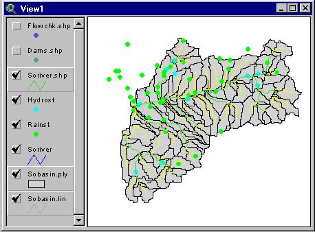
As you can see the exits of each streams have been highlighted in yellow. Check the exits manually by zooming in to make sure that all exits have been highlighted.
Some model parameters for this model need to be specified. Make the
Theme sobasin.ply active and click ![]() to view the attribute table for this coverage. Scroll to the right until
you see the fields "FlowTime" and "DiffNum"
(Diffusion Number). These are theoretical parameters that determine the
time distribution of runoff at a subwatershed outlet given a daily pulse
of rain. The concept used in this model is similar to the unit hydrograph
theory. Default values for the FlowTime and DiffNum parameters have been
assigned by the pre-processing program. To calculate the correct values
of these parameters requires information about mean flow length and the
standard deviation of mean flow length. This information can be determined
from the DEM by a separate procedure involving the Flow Length function.
This computation has been done for you already. To add these resulting
parameter values to the table, add the Table "length.dbf"
to your Project. Make "length.dbf" the active Table and highlight
the field labeled "value." Now, make "Attributes of sobasin.ply"
active and highlight the field "grid-code." With this done, select
Table / Join to obtain a single, virtually joined table. Now, select
the menu item Table / Start Editing and then highlight the field
"FlowTime" and click
to view the attribute table for this coverage. Scroll to the right until
you see the fields "FlowTime" and "DiffNum"
(Diffusion Number). These are theoretical parameters that determine the
time distribution of runoff at a subwatershed outlet given a daily pulse
of rain. The concept used in this model is similar to the unit hydrograph
theory. Default values for the FlowTime and DiffNum parameters have been
assigned by the pre-processing program. To calculate the correct values
of these parameters requires information about mean flow length and the
standard deviation of mean flow length. This information can be determined
from the DEM by a separate procedure involving the Flow Length function.
This computation has been done for you already. To add these resulting
parameter values to the table, add the Table "length.dbf"
to your Project. Make "length.dbf" the active Table and highlight
the field labeled "value." Now, make "Attributes of sobasin.ply"
active and highlight the field "grid-code." With this done, select
Table / Join to obtain a single, virtually joined table. Now, select
the menu item Table / Start Editing and then highlight the field
"FlowTime" and click ![]() .
With the Field Calculator that comes up, you set new values for FlowTime
by setting [FlowTime] = [flowt] as shown below.
.
With the Field Calculator that comes up, you set new values for FlowTime
by setting [FlowTime] = [flowt] as shown below.
Repeat this procedure to set the diffusion number: [DiffNum]=[Diffn]
You also need to specify the mean flow length field -- "MFL" -- in this table because numbers in this field are used to estimate losses during overland flow. Highlight the field "MFL" and use the calculator as shown below.
We are done with this table for now. Select Table / Remove All Joins and then Table / Stop Editing . Select Yes when prompted on to save edits and then close the table.
The next step is to interpolate missing rainfall records at the rain gauging stations. Missing data in the rainfall records are usually stored as -1 or some other negative number. The procedure for interpolating missing records uses an inverse-distance weighting (IDW) scheme. The distance from the edit station to the closest gauging station is dynamically computed at run-time. The rainfall at the latter station is used to estimate the missing records. Running the interpolation program can be very time consuming particularly when there is a large set of stations with long observed records. Hence, interpolate the missing rainfall data one year at a time. Add the monthly rainfall data, mrn87.dbf to your project by selecting add from the project window.
The script which performs this interpolation is called CMPRAIN.PRE.
Click the![]() tool from the view menu bar followed by a click in the View containing
the Souss basin coverages. Click NO if the program prompts you to run a
different script and select CMPRAIN.PRE from the resulting list.
A dialog box comes up asking the user to specify the rainfall time series
table. Select mrn87.dbf by scrolling through the list of fields
presented. The linkage between the rain gage station coverage, rainst,
and the rainfall data, mrn87.dbf is established through the rain
station theme key field, rainid, and the field names in the rainfall
data file. Interpolated records are written back to the same time series
table.
tool from the view menu bar followed by a click in the View containing
the Souss basin coverages. Click NO if the program prompts you to run a
different script and select CMPRAIN.PRE from the resulting list.
A dialog box comes up asking the user to specify the rainfall time series
table. Select mrn87.dbf by scrolling through the list of fields
presented. The linkage between the rain gage station coverage, rainst,
and the rainfall data, mrn87.dbf is established through the rain
station theme key field, rainid, and the field names in the rainfall
data file. Interpolated records are written back to the same time series
table.
Each time a new period of record is to be simulated, the surplus computation
program, CMPSURP.PRE, must be run. The program takes the rainfall
from the rain stations and interpolates it to the centroid of the watershed
polygons. The amount of rainfall that would potentially become available
as runoff is determined as surplus. This surplus is computed by applying
a percentage to the total rainfall and multiplying the result by the area
of the subwatershed polygon. This results in a value of surplus rainfall
in cubic meters per second.
Start the program by clicking on the![]() tool. Choose No if the script displayed is not CMPSURP.PRE
and select CMPSURP.PRE from the resulting list of scripts. A dialog
is initiated to specify the rainfall time series, (mrn87.dbf), rain
station theme, (rainst), the watershed polygon coverage, (sobasin.ply)
and key field, (Grid_Code), and the rain station key field, (Rainid).
CAUTION: Be sure to select the Rainid as ther rain station
key field, NOT Rainst-id. The program computes the surplus
rainfall in cubic meters per second and writes the results to the psurp.dbf
file.
tool. Choose No if the script displayed is not CMPSURP.PRE
and select CMPSURP.PRE from the resulting list of scripts. A dialog
is initiated to specify the rainfall time series, (mrn87.dbf), rain
station theme, (rainst), the watershed polygon coverage, (sobasin.ply)
and key field, (Grid_Code), and the rain station key field, (Rainid).
CAUTION: Be sure to select the Rainid as ther rain station
key field, NOT Rainst-id. The program computes the surplus
rainfall in cubic meters per second and writes the results to the psurp.dbf
file.
For each watershed in the basin, there is a corresponding field in psurp.dbf. The data in this table is linked to the watersheds by field names which contain the grid_code of the watershed polygon. For example, the field in psurp.dbf containing data for the watershed polygon with grid_code 35 is GC35. These grid_codes are maintained in all the output tables throughout the model.
With some surplus flow computed, the next step is to perform the surface water simulation. The map-based surface water flow simulation model is designed to simulate surface water flow runoff based on the excess precipitation defined on the subwatersheds of a river basin. Running the simulation model generates three flow time series. PFlow(t) is associated with a subwatershed polygon and it represents the flow contribution of the polygon. FFlow(t) , and TFlow(t) are associated with the river arcs and represent flow out of the From-Node and toward the To-Node of a river arc, respectively. The use of Tflow and Fflow is an important concept because it enables flow to be interpolated to any point along a given river arc.
Two procedures can be used to run the simulation model. The first procedure
involves begins with a click on the view containing all the coverages to
activate it. The simulation dialog is then initiated by selecting SFlowSim
from under SFlwModel in the view menu bar.
The second procedure, shown here, involves running the simulation from
the program run tool. This procedure provides the user with the option
of simulating either the whole river basin or only the portion above the
selected point. With the view containing the simulation themes as an active
document, click![]() from the ViewToolBar. Now, click on a point along the river network, in
the view, and select SFlowSim.prc from the list of programs presented.
Decide between the options provided on whether to simulate either the basin
or part of it. If you use the second procedure, be sure to click directly
on the a river arc. A click outside of the river arc will resulting a message
asking you to try again.
from the ViewToolBar. Now, click on a point along the river network, in
the view, and select SFlowSim.prc from the list of programs presented.
Decide between the options provided on whether to simulate either the basin
or part of it. If you use the second procedure, be sure to click directly
on the a river arc. A click outside of the river arc will resulting a message
asking you to try again.
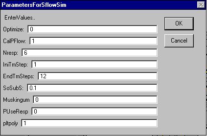
Regardless of which procedure is used to run the simulation model, a user will be presented with a multiple input table containing the model control parameters. Check the initial and final time steps (IniTmStep and EndTmStep) to ensure the period being simulated corresponds to the number of records in the output tables, in this case 12. Enter the parameter values shown in the figure above. A description of the various input parameters is provided below. The value following the equal sign of each parameter indicates the program default.
As the processing proceeds, the watershed boundary arcs are selected
and shown in red.
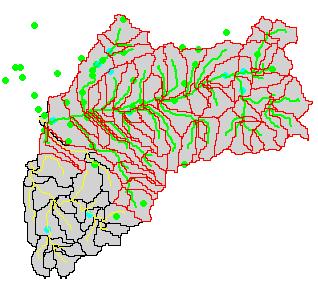
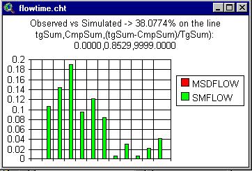
When the simulation is complete, you will be prompted on whether or not
the flow path should be selected. Your results should look like this:
To plot the flow distribution, click on ![]() in the View Tool Bar. Options for either plotting flow distribution along
a selected stream or flow time-series at a location are presented. If the
longitudinal flow profile is selected, a user can then click any location
on the river stream network to plot the longitudinal flow profile along
the river selected stream between the selected point and the outlet. If
a flow time series plot is selected, when the user click at a location,
the user is prompted to select if FFlow(t), TFlow(t), PFlow(t), or SurpFlow(t)
will be plotted. For this exercise, select 2 to plot the longitudinal
flow profile, and then click on the arc of your choice.
in the View Tool Bar. Options for either plotting flow distribution along
a selected stream or flow time-series at a location are presented. If the
longitudinal flow profile is selected, a user can then click any location
on the river stream network to plot the longitudinal flow profile along
the river selected stream between the selected point and the outlet. If
a flow time series plot is selected, when the user click at a location,
the user is prompted to select if FFlow(t), TFlow(t), PFlow(t), or SurpFlow(t)
will be plotted. For this exercise, select 2 to plot the longitudinal
flow profile, and then click on the arc of your choice.
OK, you're done!!!
These materials may be used for study, research, and education, but please credit the authors and the Center for Research in Water Resources, The University of Texas at Austin. All commercial rights reserved. Copyright 1997 Center for Research in Water Resources.