Last updated 05/26/97 - GISHydro97 CD Version
Ferdi Hellweger and David Maidment

TABLE OF CONTENTS
INTRODUCTION
HECPREPRO is a GIS preprocessor for the Hydrologic
Engineering Center’s (HEC) Hydrologic Modeling System (HMS). HMS is
currently being developed by HEC as part of the NexGen program of research.
The purpose of HECPREPRO is to summarize data from a GIS system so that
they can be used as input for HMS. HECPREPRO takes a stream and subbasin
GIS layers as input data. The output data consists of an HMS Basin file.
The system is written in ARC/INFO Arc Macro Language (AML) (Version 3.1.ai)
and ArcView Avenue (Version 4.0.av).
INPUT DATA
As input stream and subbasin data layers are required. An elevation
grid is required for the ARC/INFO implementation and optional for the ArcView
implementation. The data sets have to be in the same projection and datum.
The input data has to accurately describe the hydrologic properties of
the area. Where errors occur they are due to discrepancies among the stream
and subbasin data layers.
METHODOLOGY AND PROCEDURE
The program code is oriented around identifying hydrologic elements
and their connectivity with each other. Seven hydrologic elements are identified.
They are: subbasins, sources, reaches, junctions, reservoirs, diversions
and sinks.
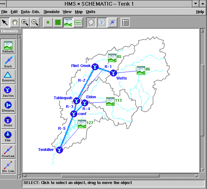
The step-by-step methodology for identifying and connecting hydrologic
elements is presented below. The data for the figures is from the Tenkiller
Reservoir drainage basin. Some features were added so that all seven hydrological
features are present. The same data is used for the sample applications
later.
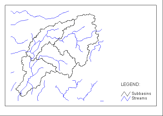
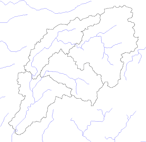
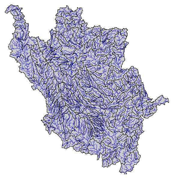
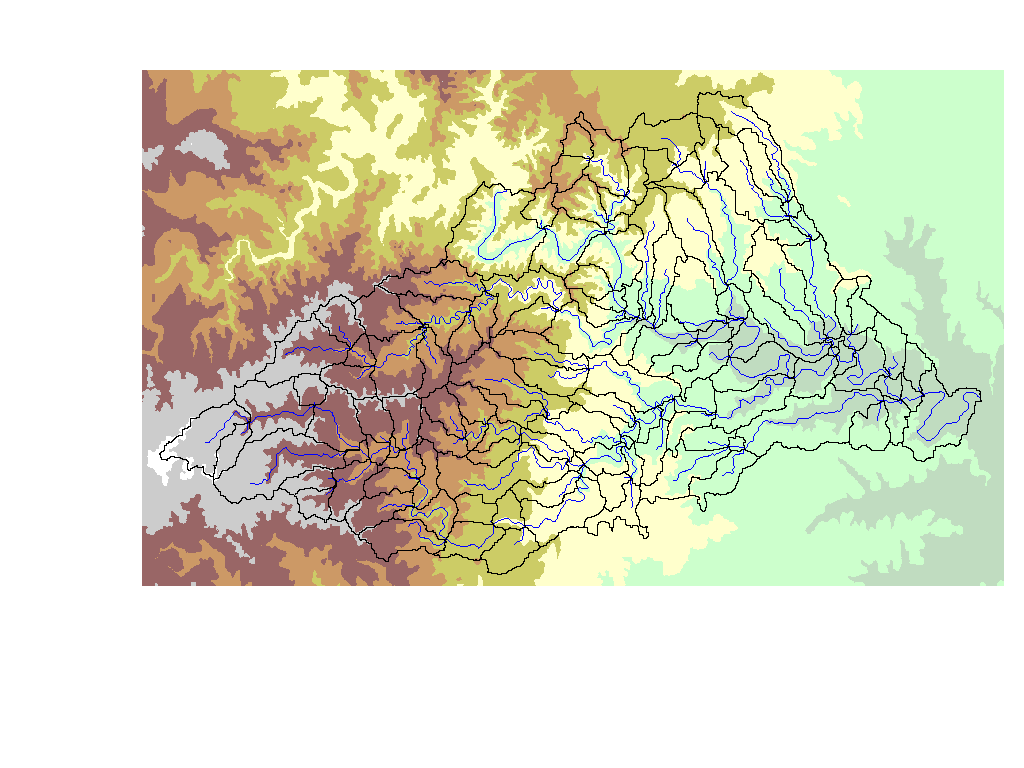
- The program starts with a stream and a subbasin data layer. The stream
and subbasin layers are shown in blue and black, respectively, in Figure
1.
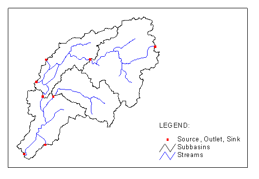
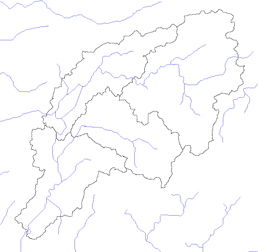
- The two layers are intersected. This removes streams outside the watershed
boundary and identifies locations at the intersection of streams and subbasin
boundaries. Those locations can represent sources, subbasin outlets or
sinks. The resulting stream layer with the intersection locations marked
in red is shown in Figure 2.
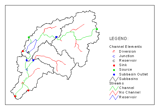
- Stream lines are classified into three types. Stream lines can be part
of the channel system that carries water from upstream features, they can
be tributaries to the channel system or they can be part of a lake or reservoir
defined by double-line connections between two channel locations.
The channel system is defined by being downstream of hydrologic elements.
There is always a source or a subbasin outlet at the most upstream end
of a channel system. That means that the channel system can also be defined
by being downstream of sources and subbasin outlets. The system identifies
the channel system by tracing downstream of the locations identified in
step 2. Reservoir lines are identified by being enclosed polygons in the
stream coverage. The channel streams (green), the non-channel streams (red)
and the reservoir streams (blue) are shown in Figure
3.
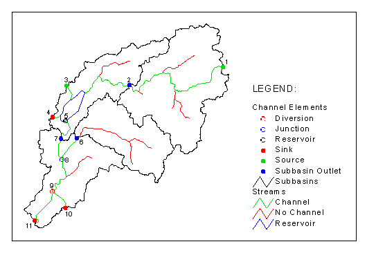
- All the elements on the channel can be identified based on their relation
to the connecting lines as follows:
Diversion - one channel line upstream and two or more channel lines downstream.
Junction - two or more channel lines upstream and one channel line downstream.
Reservoir - two reservoir lines upstream and no reservoir line downstream.
Sink - one channel line upstream and no channel line downstream.
Source - no channel line upstream and one channel line downstream.
Subbasin outlet - any intersection location not meeting the criteria for
sink or source.
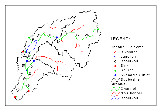
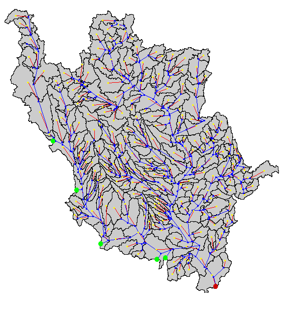
Diversions (red circles), junctions (blue circles), reservoirs (black circles),
sinks(red dots), sources (green dots), and subbasin outlets (blue dots)
are shown in Figure 4.
- A unique ID is assigned to each element on the channel system as shown
in Figure 5.
- Connectivity among channel elements is established by moving along
the channel streams from element to element. During this process multiple
stream lines are combined into single reaches and they are assigned IDs
as shown in Figure 6.
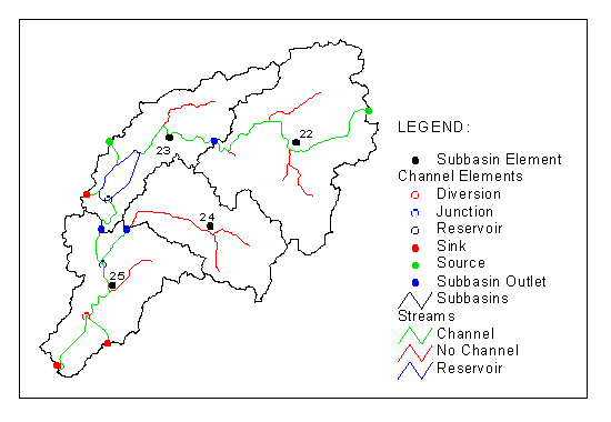
- Subbasin elements are defined by the centroid of the polygons in the
subbasin coverage. They are assigned unique IDs and marked with black dots
as shown in Figure 7.
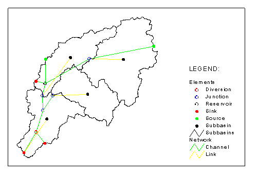
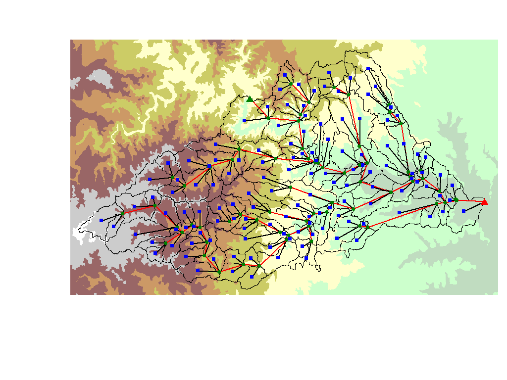
- With all the channel elements established and connectivity identified
a symbolic layer is generated. Points in the layer are diversions (red
circle), junctions (blue circle), reservoirs (black circle), sinks (red
dot), sources (green dot), and subbasins (black dot). Note that elements
previously classified as subbasin outlets are now combined with junctions,
because they serve the same function. Connection among the elements represented
by points can be with a channel (green) or a link (yellow) as shown in
Figure 8.
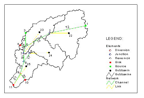
- The IDs are carried over into the symbolic layer as shown in Figure
9.
OUTPUT DATA
The output data consists of an HMS basin file, and a ‘hydrologic’ and
a symbolic data layer.
HMS Basin File
The HMS basin file is an ASCII file designed to be read by HMS directly.
Here is an example.
Hydrologic Data Layer
A ‘hydrologic’ data layer is created. The main purpose of the layer
is to serve as a working layer to store data and perform calculations during
the program run. However, the layer is also useful for trouble shooting
purposes.
Symbolic Data Layer
A symbolic data layer is created. The main purpose of the layer is
for the user to check the results of the system.
GETTING THE SYSTEM (Version 3.1.ai)
The system consists of five AML programs. The programs can be viewed
and downloaded by clicking on the hyperlinks for each program below. Alternatively
the programs can be downloaded via anonymous ftp from ftp.crwr.utexas.edu/pub/crwr/gishydro/hecprepro.
The programs and data are also on the GISHydro97 CD-ROM in directory \gishyd97\prepro\gisfiles.
REQUIRED:
hecprepro.aml
(via ftp) - main program (arc).
hecpause.aml
(via ftp) - pause utility (any).
OPTIONAL:
hecshell.aml
(via ftp) - user interactive data input shell (arc).
hechydro.aml
(via ftp) - program that reproduces hydrocov display (arcplot).
hecsym.aml
(via ftp) - program that reproduces symcov display (arcplot).
Attention PC CD Users:
The files on the CD are read-only. To run the exercise you will need
to copy the files to the hard drive of your computer or another location
where you have write permission. When doing so it is best to use the DOS
XCOPY command (rather than drag-and-drop in Windows). Using this command
will make sure the files are not marked as read-only after you copied them.
Follow these steps to copy data from the CD:
- Go to DOS.
- Go to the CD drive.
- Change to the module directory (i.e. terrain, prepro)
- Type: xcopy gisfiles destination_path /E
Attention CD Users: The programs are also located on the CD in the
prepro/gisfiles directory.
USING THE SYSTEM (Version 3.1.ai)
The system is designed to run without user interaction. This means that
the main task of the user is to start the system. The easiest way to start
the system is to use the user interactive data input shell (hecshell.aml).
The program should be run from the 'Arc'-prompt with the arc &RUN directive.
The program will prompt you for the data needed.
There are several advanced options which can control program run. They
are:
- User Observation Level
The program is designed to run, which means that if there are errors
in the input data the program will continue to run unless the error is
so severe that an Arc/INFO error occurs. The user can specify a user observation
level which controls how often the program will pause during processing.
The user observation level can be changed at each pause by typing in the
new observation level. Valid user observation levels are:
- 0 - no pause and no graphic display (for background running)
- 1 - pause at error
- 2 - pause at error and legends
- 3 - first level debug
- 4 - second level debug
- 0.10, 0.20, etc. - makes first pause at STEP 10, STEP 20, etc.
- 9 - at the pause prompt quits instantly
- Attribute Collection
Since the program code is oriented around defining hydrologic elements
and their connectivity the user has the option to bypass the collection
of attributes. If the attributes are not collected the output file will
only contain the connectivity attributes (hecid, hecupid and hecdnid).
- Prior Clipping or Intersecting
If the stream coverage was clipped or intersected with polygons from
the subbasin coverage the program has to use a slightly different method
to identify the channel system. The user can specify this during input.
- Node Snapping
Nodes from the stream coverage can be snapped to nodes from the subbasin
coverage. This is useful for data created with GRID routines. If node snapping
is to be done the user has to specify a tolerance distance to be used (which
should be set with grid size in mind).
A more detailed discussion on using the system is provided in the User's
Guide and Reference Manual.
SAMPLE APPLICATION (Version 3.1.ai)
The Tenkiller Reservoir drainage basin was used to develop the system
and serves as input data for the sample application. The sample application
can can be run on either one of two stream coverages:
- tkst1 - the actual, unmodified stream coverage
which is relatively simple.
- tkst2 - a modified, synthetic stream coverage
which has the following features added: source, diversion out of a reach,
reservoir, junction into a reservoir, diversion out of a reservoir. This
is the data used to present the methodology and procedure earlier.
To run the program follow these steps:
- Create a subdirectory called 'tk' on your computer.
- Download the above AMLs from our anonymous ftp site (ftp.crwr.utexas.edu).
They are located in the '/pub/crwr/gishydro/hecprepro' directory. Attention
CD Users: The programs are also located on the CD in the prepro/gisfiles
directory. Put the AMLs in your 'tk' directory.
- Download the tksub.e00, tkst1.e00, tkst2.e00 and tkelev.e00 files from
our anonymous ftp site. The files are in the '/pub/crwr/gishydro/hecprepro/sample/input'
directory. Attention CD Users: The coverages are also located on the
CD in the prepro/gisfiles directory. Put the files in your 'tk' directory.
- Import the coverages using the Arc/INFO IMPORT command. Note that the
tksub, tkst1 and tkst2 files are ARC/INFO coverages. The tkelev file is
an ARC/INFO grid. Attention CD Users: The coverages on the CD are not
in export format.
- Run the hecshell.aml program from within Arc with the '&run' directive.
The program will ask you for the input data one by one. Answer the questions
as follows:
Stream Coverage (required): tkst1 (or tkst2)
Subbasin Coverage (required): tksub
Elevation Grid (required): tkelev
User Observation Level: 2
Attribute Collection?: Y
Clipped?: N
Node Snapping?: N
Name of General Text File: gentkst1.txt (or gentkst2.txt)
DXF File: Y
Name of DXF File: dxftkst1.dxf (or dxftkst2.dxf)
HMS Basin File: Y
Name of HMS Basin File: hmstkst1.txt (or hmstkst2.txt)
- The program will pause at two locations, where it will also display
legends in the terminal window. To continue, just hit 'enter' when you
are ready.
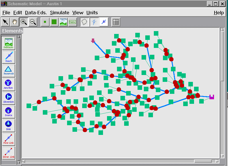
Once the program is done check the output you created. You can move
around the map with the MAPEXTEND command. To reproduce the symcov display
run hecsym.aml. Here is what your output files should look like:
If you don't have HMS here is what you would
see. Output coverages for tkst1 and tkst2 are located on the ftp site as
well.
Attention PC CD Users:
The files on the CD are read-only. To run the exercise you will need
to copy the files to the hard drive of your computer or another location
where you have write permission. When doing so it is best to use the DOS
XCOPY command (rather than drag-and-drop in Windows). Using this command
will make sure the files are not marked as read-only after you copied them.
Follow these steps to copy data from the CD:
- Go to DOS.
- Go to the CD drive.
- Change to the module directory (i.e. terrain, prepro)
- Type: xcopy gisfiles destination_path /E
SAMPLE APPLICATION (Version 4.0.av)
The Tenkiller Reservoir drainage basin was used to develop the system
and serves as input data for the sample application. The sample application
can can be run on either one of two stream layers:
- tkst1 - the actual, unmodified stream layer
which is relatively simple.
- tkst2 - a modified, synthetic stream layer
which has the following features added: source, diversion out of a reach,
reservoir, junction into a reservoir, diversion out of a reservoir. This
is the data used to present the methodology and procedure earlier.
Note: If you are new to ArcView you might want to do the exercise
entitled Introduction to ArcView.
To run the program follow these steps:
- Create a subdirectory called 'tk' on your computer.
- Download the prepro.apr project file from our anonymous ftp site (ftp.crwr.utexas.edu)
(using ASCII data transfer). It is located in the '/pub/crwr/gishydro/hecprepro'
directory. Attention CD Users: The project are also located on the CD
in the prepro/gisfiles directory. Put the project in your 'tk' directory.
- Download the following shape files from files from our anonymous ftp
site (using binary data transfer).
tksub.shp, .shx, .dbf
tkst1.shp, .shx, .dbf
tkst2.shp, .shx, .dbf
The files are in the '/pub/crwr/gishydro/hecprepro/sample/input' directory.
Attention CD Users: The shape files are also located on the CD in the
prepro/gisfiles directory. Put the files in your 'tk' directory.
- Start ArcView and open the prepro.apr project.
- Create a new view and add the three sample data sets.
- Run HEC-PREPRO by highlighting the tksub and tkst1 themes and clicking
on the 'P' button on the View's Button Bar. The program will ask you for
the run control parameters. Supply the following:
Transfer Attributes (y/n): no
HMS File Path (default, path): default
Tolerance: 10
User Observation Level (0-4): 3
Once the program is done check the output you created. Try running the
program with the tkst2 stream layer. Here is what your output files should
look like:
If you don't have HMS here is what you would
see. Output shape files for tkst1 and tkst2 are located on the ftp site
as well.
Note that the system has attribute transfer capabilities which you might
want to check out. See the user's
guide for a detailed description.

Attention PC CD Users:
The files on the CD are read-only. To run the exercise you will need
to copy the files to the hard drive of your computer or another location
where you have write permission. When doing so it is best to use the DOS
XCOPY command (rather than drag-and-drop in Windows). Using this command
will make sure the files are not marked as read-only after you copied them.
Follow these steps to copy data from the CD:
- Go to DOS.
- Go to the CD drive.
- Change to the module directory (i.e. terrain, prepro)
- Type: xcopy gisfiles destination_path /E
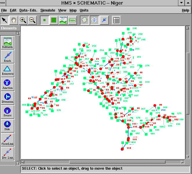
EXCITING SUCCESS STORIES
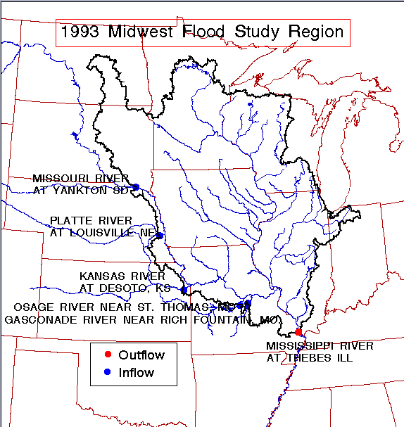
1993 Midwest Flood Region (Upper Mississippi and Missouri Basins):
Austin Project Region:
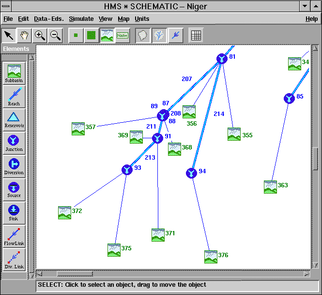
Niger River Basin:
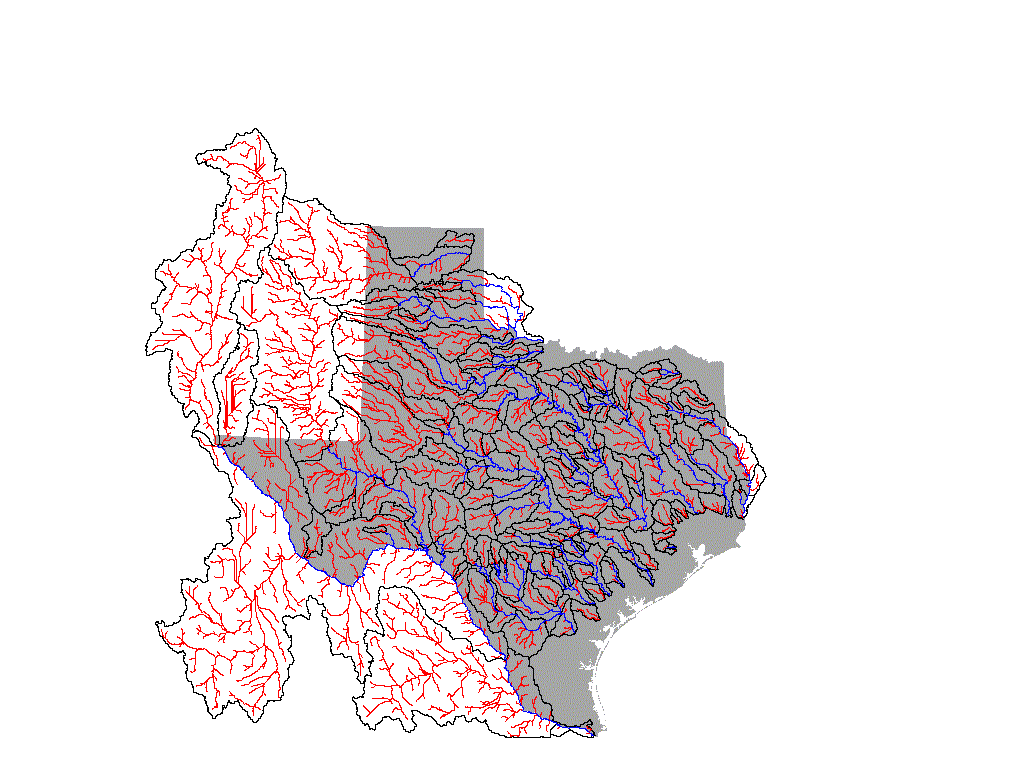
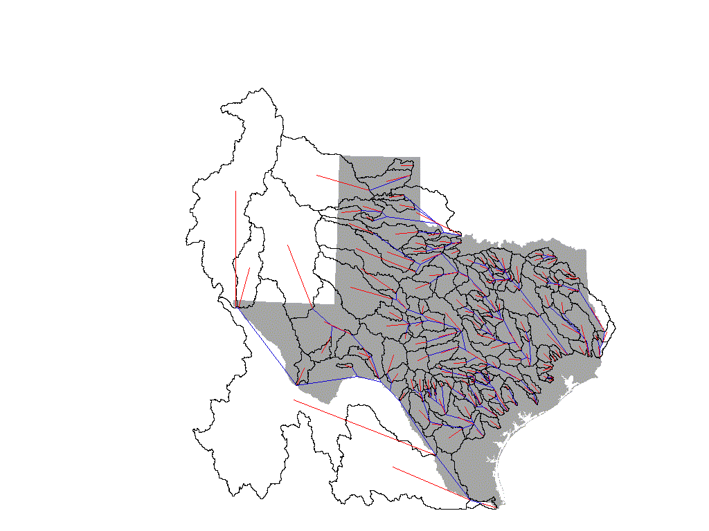
Texas:
ACKNOWLEDEGMENTS
This research was sponsored by the Hydrologic Engineering Center , US
Army Corps of Engineers, Davis, California. Their support is gratefully
acknowledged. The seven elements in the conceptual model were proposed
by John Peters.
These materials may be used for study, research, and education, but
please credit the authors and the Center for Research in Water Resources,
The University of Texas at Austin. All commercial rights reserved. Copyright
1997 Center for Research in Water Resources.
