CE 374K Hydrology Homework Assignment on

Flood Frequency Analysis

The attached spreadsheet guadalupe.xls and comma separated file guadalupe.csv contain the annual maximum discharges of the Guadalupe River at Victoria for the period 1935 – 2002. These data are also obtainable in the LRC in /class/maidment/ce374k00. Actually these data are for water years, which begin on October 1 of the previous year and continue to September 30 of the current year. These data were obtained from the Peak Flow file at http://waterdata.usgs.gov/tx/nwis/peak for USGS Station 08176500.

The data for 1935 to 1998 are plotted below. In October 1998, an enormous flood occurred on the Guadalupe River (in the 1999 water year) for which the discharge has been estimated by the USGS as being 466,000 cfs. This is not shown on the graph below to avoid making all the other floods seem very small.

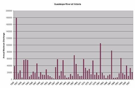
(1) Plot a graph of all the data, including the flows in 1999 and 2002.

(2) Estimate the return period of annual maximum discharges which exceed 30,000, 40,000, 50,000, and 60,000 cfs directly from the data by looking at the recurrence interval between flows exceeding those magnitudes in the data from 1935-2002.

(3) Take the logs to base 10 of the data and calculate their mean, standard deviation and coefficient of skewness for the data from 1935 – 1998, and also including the last four years of data, i.e. 1935-2002.

(4) Estimate the 100 year flood on the Guadalupe River using the Log normal (if coefficient of skewness ~ 0) or Log Pearson III method (if coefficient of skewness is significant). By how much does the inclusion of the October 1998 flood increase the 100 year flood estimate?

This assignment is due on Tuesday April 27

Annual Maximum Discharges of Guadalupe River at Victoria
Date of Occurrence	Year	Peak Discharge (cfs)
6/20/1935	1935	38500
7/3/1936	1936	179000
10/4/1936	1937	17200
4/30/1938	1938	25400
6/6/1939	1939	4940
7/3/1940	1940	55900
5/3/1941	1941	58000
7/9/1942	1942	56000
10/21/1942	1943	7710
6/1/1944	1944	12300
4/6/1945	1945	22000
9/3/1946	1946	17900
10/17/1946	1947	46000
5/28/1948	1948	6970
4/30/1949	1949	20600
10/28/1949	1950	13300
6/8/1951	1951	12300
9/16/1952	1952	28400
5/4/1953	1953	11600
10/26/1953	1954	8560
5/22/1955	1955	4950
5/18/1956	1956	1730
5/2/1957	1957	35300
2/26/1958	1958	58300
4/15/1959	1959	10100
7/1/1960	1960	23700
6/22/1961	1961	55800
11/17/1961	1962	10800
2/21/1963	1963	4100
11/11/1963	1964	5720
2/21/1965	1965	15000
12/8/1965	1966	9790
9/21/1967	1967	70000
1/25/1968	1968	44300
4/13/1969	1969	15200
5/20/1970	1970	9190
9/12/1971	1971	9740
5/16/1972	1972	58500
6/17/1973	1973	33100
10/16/1973	1974	25200
5/29/1975	1975	30200
4/19/1976	1976	14100
4/24/1977	1977	54500
9/14/1978	1978	12700
5/12/1979	1979	19300
5/19/1980	1980	11600
9/2/1981	1981	105000
5/19/1982	1982	18500
11/20/1982	1983	10900
10/21/1983	1984	3280
4/21/1985	1985	10600
11/29/1985	1986	13700
6/7/1987	1987	83400
11/28/1987	1988	3900
5/21/1989	1989	4280
9/12/1990	1990	5230
4/5/1991	1991	17000
12/25/1991	1992	61500
6/30/1993	1993	17700
5/19/1994	1994	13300
10/19/1994	1995	39600
9/22/1996	1996	9760
4/4/1997	1997	32700
10/13/1997	1998	20600
10/20/1998	1999	466000
6/12/2000	2000	6220
9/3/2001	2001	39300
7/10/2002	2002	71700