Introduction
to HEC-HMS on Waller Creek
CE 374K Surface
Water Hydrology
University Texas Austin
Prepared by David R. Maidment
Table of Contents
- Goals of the Exercise
- Obtaining the Program and the Data
- Procedure
- 1. Importing a Basin Model
- 2. Editing a Basin Model
- 3. Creating a Meteorologic Model
- 4. Defining the Control Specifications
- 5. Executing an HEC-HMS Model
- 6. Viewing HMS Results
- Waller Creek diversion tunnel design discharge
Goals of the Exercise
The intent of this exercise is to introduce you to the structure and some of the functions of the HEC-Hydrologic Modeling System (HEC-HMS), by simulating the runoff hydrographs resulting from a design storm on Waller Creek in Austin, Texas. The physical parameters describing the watershed were developed previously using the CRWR-PrePro program.
Obtaining the Program and the Data
The HEC-HMS program can be obtained from the
�A user's manual is also available at this location. The program is loaded on computers in all the rooms in the LRC.
To run the model for Waller Creek, a basin file is needed to specify the physical parameters of the watershed, and a map file to give the outline of the drainage areas and creeks. These files can be downloaded from here: Waller_Ck.basin and hms.map These files can also be obtained on the /class server in the LRC under /class/maidment/ce374k00, and also can be downloaded as a zip file: waller.zip. Make a working directory on your computer and download these files into it. Esteban Azagra-Camino performed an extensive study of Waller Creek for his MS degree. You can read more about it in Esteban Azagra's Online Report. This assignment asks you to do a study of extreme discharges on Waller Creek using rainfall-runoff analysis.
Procedure
You may start the HMS by clicking on the HEC-HMS icon
![]()
Start/Programs/hms
After a few seconds, a window similar to the following image should appear:
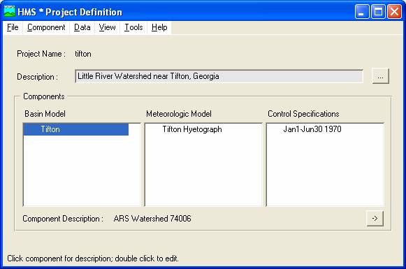
Henceforth, this image will be referred to as the Project Definition.
A Project in HMS refers to all of the data sets associated with a
particular model. In this case, the Project is called Tifton,
which is short for the Little River watershed near
In the Components section of the Project Definition, there are three sub-sections--the Basin Model, the Meteorologic Model, and the Control Specifications. Each component represents a different element of the model. The Basin Model, for instance, contains information relevant to the physical attributes of the model, such as basin areas, river reach connectivity, or reservoir data. Likewise, the Meteorologic Model holds rainfall data. Finally, the Control Specifications section contains information pertinent to the timing of the model such as when a storm occurred and what type of time interval you want to use in the model. Each of the sections is explored below individually.
1. Importing a Basin Model
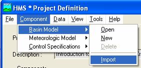
The first of the Components we will consider is the Basin Model. To create a hydrologic model of Waller Creek, we need to import the basin file that you just downloaded. In HMS Project Window, use File/New Project to open a new project by entering the following data. Notice that typing "waller" in the Project window automatically creates a subdirectory called waller in c:\hmsproj, which is where Project files are stored when HMS is executed.

In the HMS Project window, use Component/Basin Model/Import to import the basin model file Waller_Ck.basin from your working directory.
You'll see the Basin window open up and some icons appear. If a warning message appears about the length of the name Junction with Hemphill, click
OK
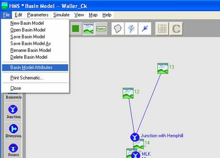
. In the HMS Basin Model window, use File/Basin Model Attributes to select the location where you have stored the HMS.map file and add to the display.
You should then see a schematic of Waller Creek showing the watershed and stream map and an overlay of the hydrologic elements.
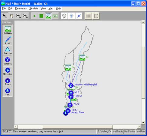
The tool bar on the left hand side of the display shows the seven hydrologic elements contained in HEC-HMS. They are:
![]() Subbasin -
rainfall-runoff computation on a watershed
Subbasin -
rainfall-runoff computation on a watershed
![]() River reach - routing of flows from one
end of a reach to the other
River reach - routing of flows from one
end of a reach to the other
![]() � Reservoir
- routing of flows through a level-pool reservoir
� Reservoir
- routing of flows through a level-pool reservoir
![]() � Junction
- combination of flows from upstream reachs and subbasins
� Junction
- combination of flows from upstream reachs and subbasins
![]() � Diversion
- abstraction of flow from the stream
� Diversion
- abstraction of flow from the stream
![]() � Source
- inflow of water from a stream crossing the boundary of the modeled region
� Source
- inflow of water from a stream crossing the boundary of the modeled region
![]() � Sink -
outflow of water in a stream crossing the boundary of the modeled region (basin
outlet)
� Sink -
outflow of water in a stream crossing the boundary of the modeled region (basin
outlet)
The model of Waller Creek shown above contains only 4 of these kinds of
elements. There are 19 hydrologic elements in the Waller Creek model,
made up of 7 subbasins, 6 river reaches, 5 junctions,
and 1 sink at the point where Waller Creek flows into the
To be turned in: a map of the Waller Creek HMS model
To screen-capture an image, do the following:
- Make sure the HMS Basin Model is the top window in your terminal.
- Depress Shift-PrntScrn on your keyboard. This captures the image on your screen and places it on the clipboard.
- Open Paint using Start/Programs/Accessories/Paint.
- In Paint, select Paste from the Edit menu. After a few seconds, the screen image should appear in the Paint window.
- Directly under the word
"File" in the Paint menu, there is a dotted rectangle
 . Make
sure this button is depressed. Enlarge the Paint window so you can see all
of the basin map. Make a rectangle around the basin map by holding down
the left mouse button and dragging. When you have completed the rectangle,
let go of the mouse button; your dotted rectangle around the basin map
should remain.
. Make
sure this button is depressed. Enlarge the Paint window so you can see all
of the basin map. Make a rectangle around the basin map by holding down
the left mouse button and dragging. When you have completed the rectangle,
let go of the mouse button; your dotted rectangle around the basin map
should remain. - Under Edit in the Paint menu, select Copy To. We are now going to save the basin map to a file.
- Change the Save as type: bar to 24 Bitmap. Type in a file name and save the file somewhere
- Open Microsoft Word.
- From the main menu in Word, select Insert/Picture/From File. Retrieve the basin image you just saved. The image should appear in your Word window.
2. Editing a Basin Model
After first making sure that the ![]() is
depressed in the Basin Model, click on the icon which represents basin
12 with the left mouse button. After this icon is highlighted, hold down the
right mouse button and choose Edit from the pop-up menu that appears. In
the upper-right-hand corner of the Subbasin
Editor window that will appear, you will find the the
area of sub-basin 12 (3.602 sq. km). Make a note of this value. Go ahead and look
up the areas of the other sub-basins as well. HMS can work with a Basin file in
either SI or English units. In this case, the file is in SI units.
is
depressed in the Basin Model, click on the icon which represents basin
12 with the left mouse button. After this icon is highlighted, hold down the
right mouse button and choose Edit from the pop-up menu that appears. In
the upper-right-hand corner of the Subbasin
Editor window that will appear, you will find the the
area of sub-basin 12 (3.602 sq. km). Make a note of this value. Go ahead and look
up the areas of the other sub-basins as well. HMS can work with a Basin file in
either SI or English units. In this case, the file is in SI units.
To be turned in: a table showing the areas of the subbasins. What is the total drainage area of Waller Creek (sq. km)?
Returning to the HMS, focus your attention on the Basin Model window.
This window contains a variety of buttons which you may use to assemble and
view a basin model. First, consider the top row of buttons. The ![]() button allows you
to select (highlight) items in the model. You may also use the
button allows you
to select (highlight) items in the model. You may also use the ![]() button to drag-and-drop
hydrologic elements from the left-hand-side of the window or to move individual
elements within the model. If you have a model element highlighted, hold down
the right mouse button and select Edit from the pop-up menu to view its
properties. The
button to drag-and-drop
hydrologic elements from the left-hand-side of the window or to move individual
elements within the model. If you have a model element highlighted, hold down
the right mouse button and select Edit from the pop-up menu to view its
properties. The ![]() button allows you to move (or pan) the entire model display by
holding down the left mouse button and moving the mouse. If you wish to zoom in
or out, you may do so by depressing the
button allows you to move (or pan) the entire model display by
holding down the left mouse button and moving the mouse. If you wish to zoom in
or out, you may do so by depressing the ![]() or
or ![]() button
respectively and selecting a rectangular area in the model to zoom in to or out
from by holding down the left mouse button and dragging the mouse to draw a
rectangle. Go ahead and experiment with these buttons to understand better how
each works.
button
respectively and selecting a rectangular area in the model to zoom in to or out
from by holding down the left mouse button and dragging the mouse to draw a
rectangle. Go ahead and experiment with these buttons to understand better how
each works.
The second set of icons under the menu bar allows you to choose how the
hydrologic elements are represented in the model. From left to right, you
choices are small symbol ![]() , large symbol
, large symbol ![]() , standard icon
, standard icon ![]() (same icons as those used on the
left-hand-side of the window), or text name
(same icons as those used on the
left-hand-side of the window), or text name ![]() . Take a minute and select each of
these buttons; notice how each button affects the model image differently.
. Take a minute and select each of
these buttons; notice how each button affects the model image differently.
Next, the third set of icons allows you to turn on or off the display of the
watershed boundaries![]() , the river reaches
, the river reaches ![]() , or flow-direction arrows
on the reaches
, or flow-direction arrows
on the reaches ![]() . As before, take some time to investigate for yourself how each
of these buttons functions. Notice that if you turn off both
. As before, take some time to investigate for yourself how each
of these buttons functions. Notice that if you turn off both ![]() and
and ![]() while
while ![]() is turned on, you
are left with a collection of icons from the elements list. In most cases, this
is how you would normally display models. For this model, however, the watershed
boundaries and the river reaches were imported earlier as an image using a
technique we will encounter in more detail later. Keep in mind that this image
has no influence on the model's output. In the final horizontal group of
buttons,
is turned on, you
are left with a collection of icons from the elements list. In most cases, this
is how you would normally display models. For this model, however, the watershed
boundaries and the river reaches were imported earlier as an image using a
technique we will encounter in more detail later. Keep in mind that this image
has no influence on the model's output. In the final horizontal group of
buttons, ![]() allows you to view a chart summarizing the results from a run, while
allows you to view a chart summarizing the results from a run, while ![]() commences
computations of a model. For the time being, do not use these buttons; we'll
come back to them later.
commences
computations of a model. For the time being, do not use these buttons; we'll
come back to them later.
At this point, click on ![]() so that the elements in the model are displayed as they are along
the left side of the window. As needed, you may drag-and-drop elements
into the model area. Go ahead and try this, but make sure you keep the elements
you add away from the elements currently in the model. Try taking a river reach
and connecting a junction to each end. To do this, grab one
so that the elements in the model are displayed as they are along
the left side of the window. As needed, you may drag-and-drop elements
into the model area. Go ahead and try this, but make sure you keep the elements
you add away from the elements currently in the model. Try taking a river reach
and connecting a junction to each end. To do this, grab one ![]() and two
and two ![]() 's. Hook up one
junction to one end of the reach by highlighting the junction (use
's. Hook up one
junction to one end of the reach by highlighting the junction (use ![]() ) and holding down the right mouse button. When the pop-up menu
appears, select Connect Downstream. Repeat these steps appropriately to
connect the stream to the other junction. To delete the elements you have added
when you are finished, highlight all added elements (hold down the shift key to
keep adding elements) and then choose Delete Elements from the Edit
menu in the Basin Model window. If you want, take some time now to
experiment with some of the other hydrologic elements.
) and holding down the right mouse button. When the pop-up menu
appears, select Connect Downstream. Repeat these steps appropriately to
connect the stream to the other junction. To delete the elements you have added
when you are finished, highlight all added elements (hold down the shift key to
keep adding elements) and then choose Delete Elements from the Edit
menu in the Basin Model window. If you want, take some time now to
experiment with some of the other hydrologic elements.
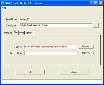
As the calculation steps above suggest, the primary function of a surface-water model such as the HMS involves three sets of calculations--quantifying rainfall losses into the soil, converting excess rainfall to runoff, and routing. As part of creating a HMS model, the selection of the processes to be used for each calculation set is made in the Basin Model Attributes window.
To access this window, select Basin Model Attributes from the File menu in the Basin Model window. The following window should appear:
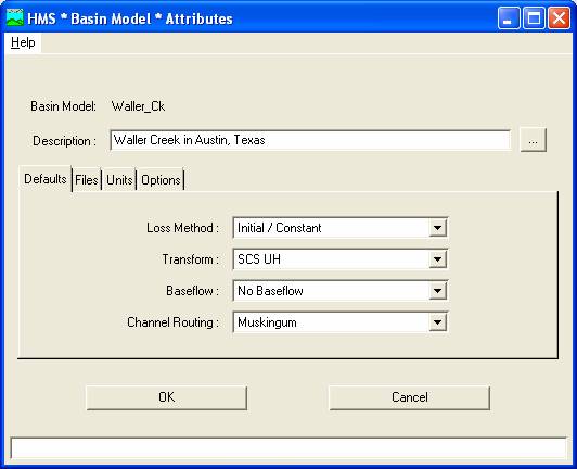
In this window, take a look at the Default Methods section. The
method on the left, Loss Rates, is where you choose the process which
calculates the rainfall losses absorbed by the ground. Click on ![]() in the Loss
Rate section to see your choices. Some options are SCS Curve No. and
Green & Ampt. In this model, Initial/Constant
has been selected. This loss relationship means that a quantity of rainfall
will be absorbed by permeable soil initially, and a constant rate will be
absorbed over the time frame of the model.
in the Loss
Rate section to see your choices. Some options are SCS Curve No. and
Green & Ampt. In this model, Initial/Constant
has been selected. This loss relationship means that a quantity of rainfall
will be absorbed by permeable soil initially, and a constant rate will be
absorbed over the time frame of the model.
The middle section, Transform, allows you to specify how to convert
excess rainfall to direct runoff. Again, click the ![]() to view
your options, most of which you should recognize. This model employs the SCS
technique. The modClark model takes gridded rainfall data, subtracts the losses as specified
through the Loss Rates, and converts the excess rainfall to a runoff hydrograph
using a variation of what is known as the
to view
your options, most of which you should recognize. This model employs the SCS
technique. The modClark model takes gridded rainfall data, subtracts the losses as specified
through the Loss Rates, and converts the excess rainfall to a runoff hydrograph
using a variation of what is known as the
The final part of the Default Methods considers Routing, which
is where you specify the process for routing a hydrograph through a river
reach. Once again, click the ![]() and look over the choices. The Muskingum
is specified here, which is the routing technique used for the reaches in this
model.
and look over the choices. The Muskingum
is specified here, which is the routing technique used for the reaches in this
model.
At this point, close the Basin Model Attributes window by clicking on
Cancel at the bottom of the window. Now that we have considered the
various loss, transform, and routing techniques to use, we will look at the
actual parameters associated with the chosen techniques. Choose Parameters/Loss Rate/Initial Constant
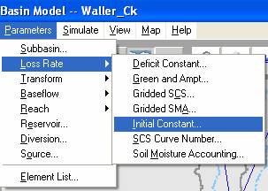
. The following window should appear.

Note that while the Initial/Constant Loss Rate method was specified via another menu, it is in this table that the method parameters are actually entered. Each basin requires an initial loss quantity, a constant loss rate, and a percent imperviousness. These values have been selected arbitrarily. If the % impervious value differs from 0, that % of the land area is assumed to have no losses and the loss method is applied only to the remainder of the drainage area
After you have looked over the data, click OK. For future reference, while both OK and Apply transfer the data to the computer's short-term memory, they differ only in that OK closes the window while Apply keeps the window open.
Once you have closed the Initial/Constant Loss window, choose Parameters/Transform/SCS to view this image:
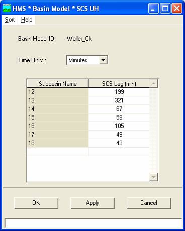
Note that the SCS unit hydrograph method requires only one parameter for each sub-basin--lag time between rainfall and runoff in the subbasin. HMS. At this point, go ahead and close this window.
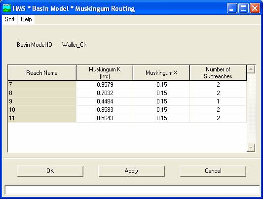
The next step involves entering the parameters for the routing process. From Parameters/ Reach / Muskingum. This should cause the following image to appear. This simulation routes the water through the reaches by the Muskingum method in which K is the travel time of a flood wave passing through the reach, X is a measure of the degree of storage (X = 0 means a level-pool reservoir or maximum storage, X = 0.5 means a pure transmission reach in which there are no storage effects, and X ranges between 0 and 0.5). The reach is divided into a number of subreaches if necessary to keep the computations numerically stable.
You do not have to go through the Parameters menu to edit element properties. Editing may also be accomplished by highlighting an element, holding down the right mouse button, and choosing Edit from the pop-up menu.
In this Paramters/Baseflow option of the HMS, you supply if necessary, information such as basin areas and initial base flows in the system. In this model we are not allowing for any base flow. close the Basin Model window by selecting Close from the File menu.
To be turned in: Choose subwatershed 14 and reach 10 and describe in words what the parameter values are that are used to characterize these hydrologic features.
3. Creating a Precipitation Model
Having established the physical aspects of the model, we will now address
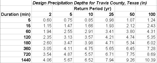
the rainfall data. From a statistical study of extreme storm rainfall
data recorded at gages, tables and maps have been prepared for the whole US
which specify the storm precipitation depth to be expected as a function of the
return period of the event and the duration of the rainfall. A table of
such values is shown below for
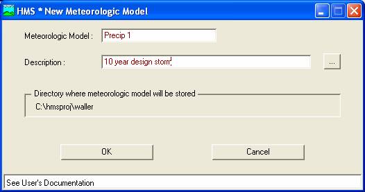
We are going to input the rainfall to HMS in English units (inches). To create a design precipitation input file, go to the Project Window and select Component/ Meteorologic Model/New. A window like this appears in which you can describe the precipitation file you intend to create, in this case for a 10 year storm.
After clicking, OK, the following window appears,
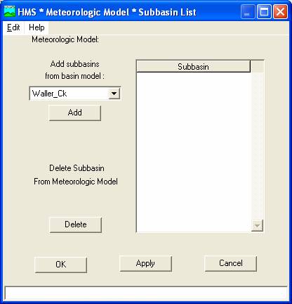
This specifies to what basin the meteorologic data are to be applied.� Click OK.
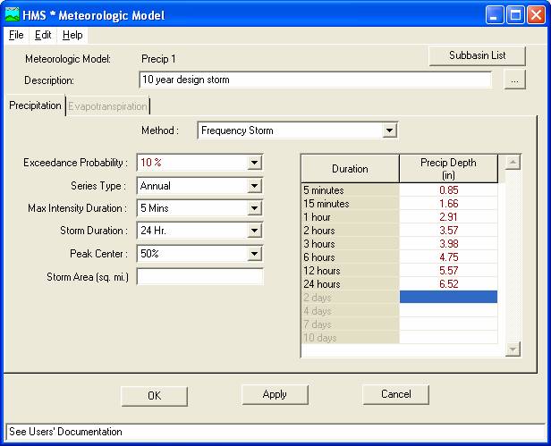
From the meteorologic model window, select Frequency storm for the User Hyetograph
Don’t worry about the warning message that then appears about losing data for another option.
When you click on Ok, the following table appears. Fill in the values shown from the table above for a 10 year storm (10% chance of being equalled or exceeded in any year). Click Apply, and then Ok to complete this step.
For each project, the HMS then creates an output Data Storage System DSS file which stores calculated data from all runs for a given project so that results from a previous run can be directly compared to results from a more current run. The HMS stores data in the DSS file according to the information given in the Pathnames section. F: is left blank because the HMS will place the name of the run there.
To be turned in: a screen capture of the design precipitation input file
4. Defining the Control Specifications
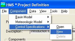
The final piece of the model setup involves establishing the model's time limits. Go back to the Project Definition and select Parameters/Control Specifications/New. The following window will appear in which you can label the specifications.
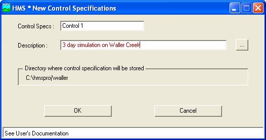
After you click Ok, you'll get the window to specify the duration of the simulation in date and time, and also the time interval of the calculations (10 minutes). In this case, the duration is arbitrary, long enough to depict the runoff from a 1-day storm, but the 10 minute time interval is part of the Basin file model setup and should remain fixed for this Waller Creek model.
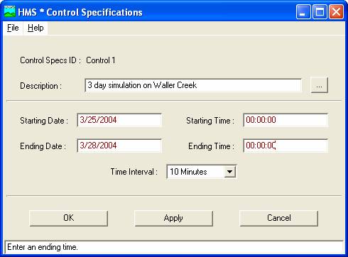
To be turned in: how many time intervals of computation will be performed?
5. Executing an HMS Model
Finally, you have finished perusing the data involved in
creating the Tenkiller model. To run the model, go
the HMS Basin Model window and select Compute <Run 1>
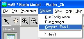
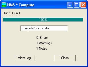
You should get a window that says the following:
If you want to make runs with alternative model files, you
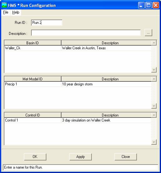
�Run Configuration from the Simulate menu. The following window should appear. Click on each of the three boxes to highlight and select them, hit Add to record these as the files to be used for Run 2, and Close the window. The three subsections in this window list the physical, rainfall, and timing data sets that have been created for this project. Though this model only has one data set in each section, the HMS is slick in that it allows the user to have multiple data sets available to include conveniently in different runs.
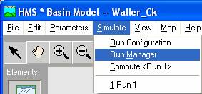
Close the Run Configuration window, go back to the Basin Model, and choose Simulate / Run Manager. You should see an image similar to this: which shows what files were used on this Run.
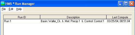
If you do not see this window, problems have arisen. If so, HMS gives a list of problem locations and by editing the Basin file you may be able to eliminate them.
6. Viewing HMS Results
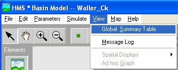
The HMS allows you to view results in tabular or graphical form. To view a global results table, go to the Project Definition and double-click WallerCk . From the window which appears (the Basin Model window), go to View and choose Global Summary Table. You'll get a window like that shown below which summarizes the peak discharge and time, the total volume of storm runoff and the drainage area from which it came.

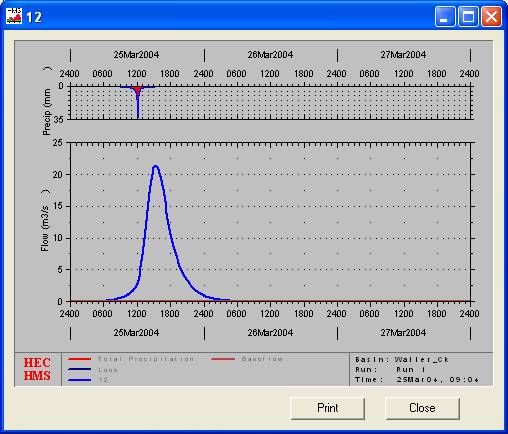
In addition to viewing global results, you may also view results for each
element within the model. To do this, choose ![]() in the Basin Model window,
select an element in the model (
in the Basin Model window,
select an element in the model (
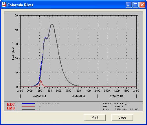
The light red hydrograph is the inflow data from the small area of Waller
Creek immediately upstream of the
To be turned in: Make a table showing the peak discharge in cms at each of the six outlet points on Waller Creek (5 junctions and 1 sink).. What is the drainage area above each of these points? What is the peak discharge per unit of drainage area (cms/sq. km) for these points?
Waller Creek Diversion Design Study
The citizens of
Recompute the flows from the HMS model using the
100 year design storm instead of the 10 year design storm.�� How much water would have to be diverted at
Recompute the flows from the HMS model using a
2-year, 5-year, 25-year, and 50-year storms.��
Make a plot showing the peak discharge to be expected from these events
at
To be turned in: A graph and a table showing the
relationship between flood peak discharge and return period for Waller Creek at
15th St.�� Determine the flow
diversion needed at
Go to Dr Maidment's Home Page