CE
374K Hydrology Developing
Steady-State Simulations in HEC-RAS
The goal of this section is to develop the HEC-RAS model for Waller Creek. The model’s geometry data and steady flow data is provided for you in the wallerras.zip file. This file can also be obtained at \class\maidment\ce374k00 in the LRC server. The geometry file was developed from GeoRAS and imported as a HEC RAS Import File. The steady flow file was extracted from a HEC HMS hydrologic model and is shown in HMSResults.xls. The process is divided in two steps:
- Open the geometry and steady flow data by opening the HEC RAS project file, waller1.prj.
- Run a steady flow simulation and export the results of the simulation into Arcview using the GeoRAS post-processor.
Geometry Data
To open HEC-RAS, look for a folder called “HEC” from the Start button on your computer, there should be a HEC-RAS 2.1, HEC-RAS 2.2, or HEC-RAS icon. Double click the icon to open the main project window, which looks like this:
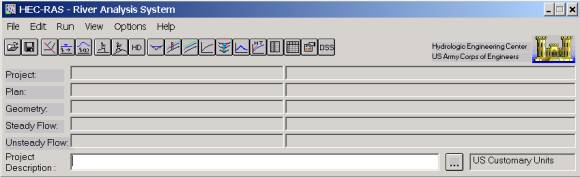
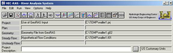
When you extracted the files from georas.zip, the HEC RAS files (waller1.prj, waller1.g02, waller1.f01) should currently be in your working directory. Click on the Open Project… command from the File menu. Scroll down to your working directory and highlight the project titled “Use of GeoRAS Input”, file waller1.prj. Click OK. The Project, Geometry, and Steady Flow information lines should now be filled with the titles of those respective files as shown:
As shown in the main menu, four files are required to run a HEC-RAS project. First, the Project File acts as a file management tool and identifies which files are used in the model. The Plan File sets the model conditions as subcritical, supercritical, or mixed flow and runs the simulation. The Geometry File contains all the geometric attributes for the model (which, for our case, are imported from GIS using GeoRAS). Lastly, the Steady Flow File establishes the steady-state flow and boundary conditions at numerous points in time for the model. (If you are using HEC-RAS 3.0, you will have a row in the main menu for Unsteady Flow. Disregard the Unsteady Flow information line and continue with the exercise.)
Geometry Data
Let’s first examine the geometry data that was developed using the same methodology we used in the previous section. Select Edit/Geometric Data… from the main project window. You should have the Geometric Data editor appear:
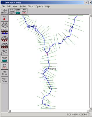
Additional editing of Geometry Data is accomplished from this window. Click on the Cross Section button to see the tabular data for each cross section. Control structures along a stream can be manually entered using the corresponding buttons from this editor. We will not be using any control structures for this model. From the Cross-section menu, choose Plot to plot the Cross-section Use File/Copy to Clipboard to save your cross-section plot.
Select File/Save Geometry Data and then File/Exit Geometry Data Editor. You will be back to the main project window. We are now ready to input the flow data for the model.
To be turned in: Take the
Cross-section whose results you described previously and make a plot of the
cross-section. How wide is the cross-section in feet? What Manning’s “n” values have been used at this
cross-section? At what distance (ft)
from the left end of the cross-section are the left and right banks?
The flow data has been extracted from a HEC-HMS hydrologic model of the Waller Creek Basin. The flow data is in cubic feet per second (cfs) and is derived from a 100-yr design storm for the Austin area. For reference only, the data is also provided for you in the MS spreadsheet, HMSResults.xls.
First, let’s open the Steady Flow Editor. Select the Steady Flow Data… command from the Edit menu. The Steady Flow Editor should look like the following:
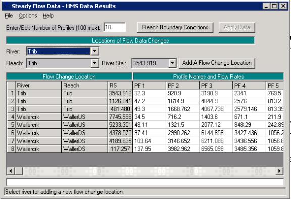
There are three sections of Steady Flow Data that has been inputted using this window: Enter/Edit Number of Profiles, Flow Change Location/Profile Names and Flow Rates, and Reach Boundary Conditions.
Enter/Edit Number of Profiles
A “Profile” is a list of flow conditions at specified locations along the extent of the model’s reaches at a specified point in time. Each entered Profile will calculate a steady-state water surface elevation along the length of each reach. Open completion of running the model (which we will do in the next section) results can be observed from the View Profiles, View Cross Sections, or View 3D Multiple Cross Section Plot buttons provided in the HEC-RAS Main Menu window.
For this exercise, a total of ten profiles were entered. The profiles correspond with flow data extracted from the HMSResults.xls file at one-hour time intervals, at 0100 hours, 0200 hours, 0300 hours, and so on, for Decemeber 1, 1999.
Open Flow Data
The editor initially showed the upstream cross sections of each reach in the model: cross sections 3543.919 (upstream boundary of the Tributary), 7745.596 (upstream boundary of WallerUS), and 4378.570 (upstream boundary of WallerDS). In addition, the cross sections acting as outlets of watersheds for rainfall runoff were added as well. If you examine the spreadsheet, HMSResults.xls, you will find flow data for upstream boundaries as well as runoff data for specified cross sections along both Waller Creek and the Tributary. This data was used for this model. When adding the flow data to HEC-RAS, the values entered for a specified cross section is an accumulated flow. All flows upstream of a flow change location in the model must be added to the flow at that point. In other words, the model is obtaining a “snapshot” in time of the flow at locations along each reach to develop the water surface profiles.
Reach Boundary Conditions
The final step in the Steady Flow Data development is establishing the Reach Boundary Conditions. Click on the Reach Boundary Conditions button. The Steady Flow Boundary Conditions Editor is used to set the water surface elevation boundary conditions. Click in the “Known WS” cell in the Downstream column. Notice that the water surface elevation for cross section 14.035 on “WallerDS” is inputted for each profile, establishing the boundary conditions for each steady-state profile.
HEC-RAS Steady Flow Simulation
We are now ready to run a Steady-State Flow simulation. From the Simulate or Run menu, select Steady Flow Analysis. Under the File menu, select New Plan. Enter “Hypothetical flow conditions” as the Plan’s title and put into the next window which appears a 12-character short identifier, “Hypoflow”. Click OK.
Ensure the Flow Regime is set to Subcritical and press the COMPUTE button. This starts a FORTRAN program called SNET, which carries out all the calculations for the simulation. A DOS window with a message indicating the end of the process will appear when the computations are completed. Close the DOS window by clicking the Close button in the upper right corner.
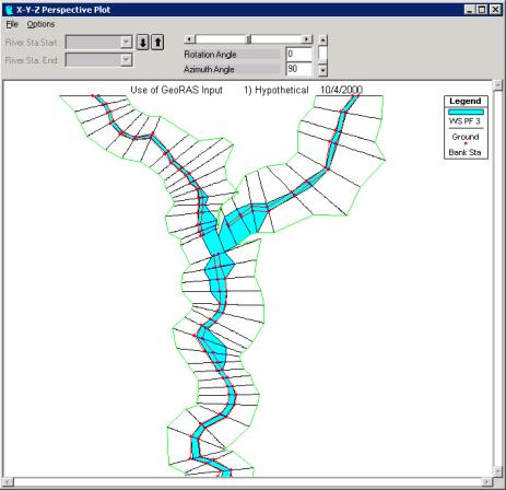
You can see the results of the model using the 3D Multiple Cross Section
plot button. Click on the ![]() button.
Under the Options menu, click on Reaches… Click on the Select All button
and then click OK. Adjust the
Rotation and Azimuth Angles to see the attributes of the buildings in the cross
sections. Choose different profiles by
clicking on Profiles.. under the Options menu. This is what Profile #3 should look like:
button.
Under the Options menu, click on Reaches… Click on the Select All button
and then click OK. Adjust the
Rotation and Azimuth Angles to see the attributes of the buildings in the cross
sections. Choose different profiles by
clicking on Profiles.. under the Options menu. This is what Profile #3 should look like:
Select File/Exit to return to the HEC-RAS main window.
To be turned in: A 3-D profile plot of the computed water surface elevation for Profile 3. (You can use File/ Clipboard to copy the plot in the X-Y-Z perspective plot window)