Introduction to HEC-HMS on Waller
Creek
CE 374K Surface Water Hydrology
University of Texas at Austin - Spring, 2011
Prepared by David R. Maidment and Gonzalo Espinoza
Table of Contents
- Goal of the Exercise
- Obtaining the Program and the Data
- Procedure
- 1. Importing a Basin Model
- 2. Editing a Basin Model
- 3. Creating a Meteorologic Model
- 4. Defining the Control Specifications
- 5. Executing an HEC-HMS Model
- 6. Viewing HMS Results
- Waller Creek diversion tunnel design discharge
Goal
of the Exercise
The intent of this exercise is to introduce you to the structure and some of the functions of the HEC-Hydrologic Modeling System (HEC-HMS), by simulating the runoff hydrographs resulting from a design storm on Waller Creek in Austin, Texas.
Obtaining
the Program and the Data
The HEC-HMS Version 3.5 program can be obtained from the Hydrologic Engineering Center at http://www.hec.usace.army.mil/software/hec-hms/ A user's manual is also available at this location. The program is loaded on computers in the LRC room ECJ 3.302. You may choose to do this homework on your own computer or in the LRC.
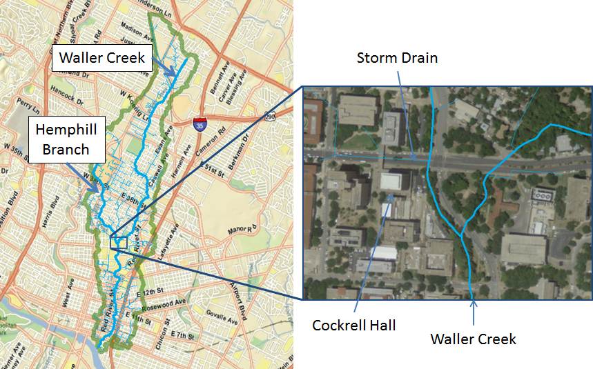
Here is a map of Waller Creek so you can see its relation to the University of Texas campus and to Cockrell Hall.
To run the HEC-HMS model for Waller Creek, a basin file is needed to specify the physical parameters of the watershed, and a map file to give the outline of the drainage areas and creeks. These files can be downloaded from here http://www.caee.utexas.edu/prof/maidment/CE374KSpring2011/HMS/waller.zip as a zip file. Make a working directory on your computer and extract these files (Waller_Ck.basin and hms.map) into it.

Procedure
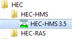
You may start the HMS by clicking on the HEC-HMS icon
Start/All Programs/HEC/HEC-HMS
If you are using HEC-HMS on your own computer for the first time, you’ll have to agree to some conditions of use of the program. You have to scroll down through these conditions before you will be able to Accept them.
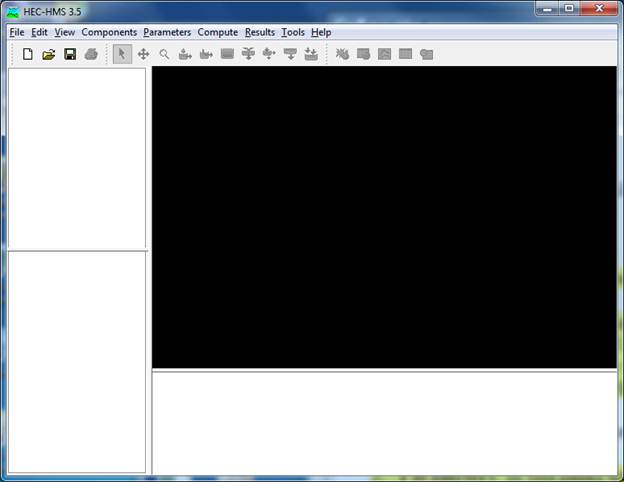
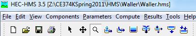
Once HEC-HMS opens, you’ll see the following screen:
1.
Importing a Basin Model
The first of the Components we will consider is the Basin Model. To create a hydrologic model of Waller Creek, we need to import the basin file that you just downloaded. In HMS Project Window, use File/New to open a new project by entering the following data

A Project in HMS refers to all of the data sets associated with a particular model. The Description bar underneath the Project name allows you to type a detailed name for the actual short Project name.
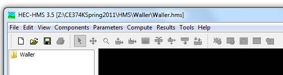
Notice that after creating the new project, a new folder called “waller” is created inside the location chosen, and the Main Window appears as:
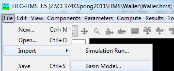
In the HMS Main Window, use File/Import/Basin Model… to import the basin model file Waller_Ck.basin from your working directory.
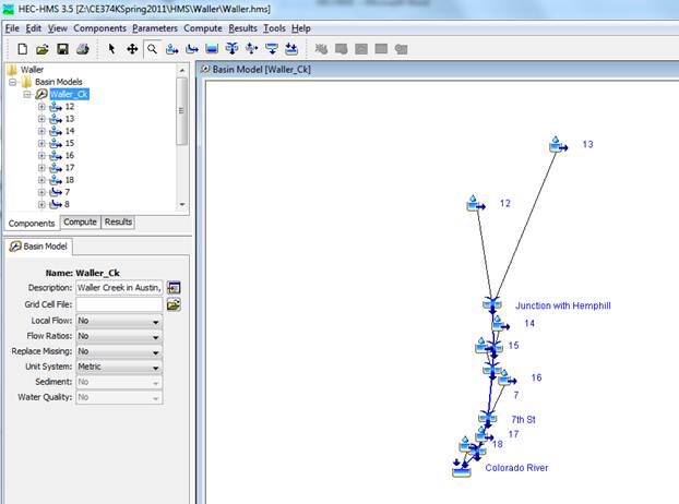
You'll see in the waller folder a subfolder called Basin Models in the Data Panel on the left hand side of the HMS model display, expand it and select Waller_Ck, the Basin window open up and some icons appear.
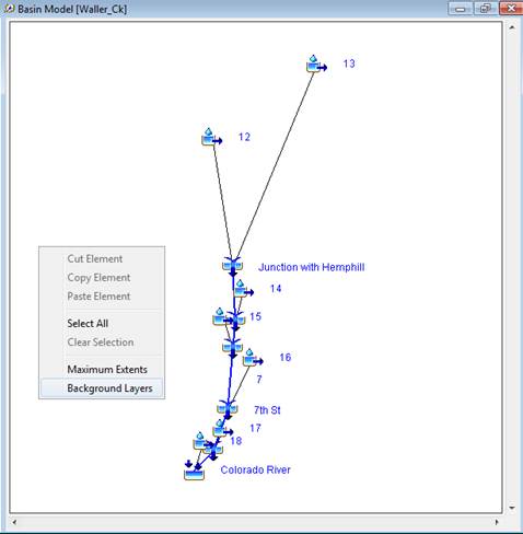
Right click in an empty area of
the Basin Model Window, select Background Layers
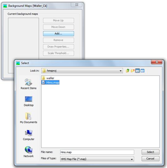
A new window will appear, click Add... change the Files of type option to HMS Map File (*.map) and select Hms.map from your working directory.
![]()
![]()
![]()
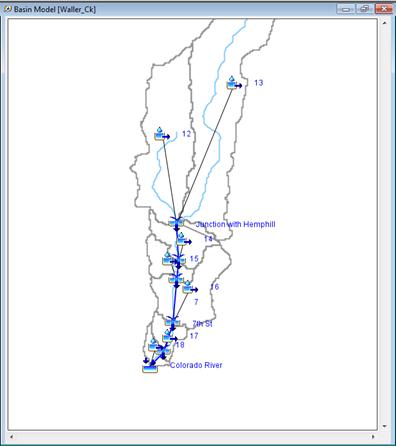
You should then see a schematic of Waller Creek showing the watershed and stream map and an overlay of the hydrologic elements in the Basin Model Panel
In the HMS menu there are displayed the seven hydrologic elements contained in HEC-HMS.
They are:
![]() Subbasin -
rainfall-runoff computation on a watershed
Subbasin -
rainfall-runoff computation on a watershed
![]() River reach - routing of flows from one
end of a reach to the other
River reach - routing of flows from one
end of a reach to the other
![]() Reservoir
- routing of flows through a level-pool reservoir
Reservoir
- routing of flows through a level-pool reservoir
![]() Junction
- combination of flows from upstream reachs and subbasins
Junction
- combination of flows from upstream reachs and subbasins
![]() Diversion
- abstraction of flow from the stream
Diversion
- abstraction of flow from the stream
![]() Source
- inflow of water from a stream crossing the boundary of the modeled region
Source
- inflow of water from a stream crossing the boundary of the modeled region
![]() Sink -
outflow of water in a stream crossing the boundary of the modeled region (basin
outlet)
Sink -
outflow of water in a stream crossing the boundary of the modeled region (basin
outlet)
The model of Waller Creek shown above contains only 4 of these kinds of elements. There are 18 hydrologic elements in the Waller Creek model, made up of 7 subbasins, 5 river reaches, 5 junctions, and 1 sink at the point where Waller Creek flows into the Colorado River. Notice that when a stream flows through a watershed, the additional local runoff from the drainage area around the stream is not accounted for until the downstream end of the reach where its flow is combined at a junction with the flow coming from the upstream reach. The junctions have been located at points where roads cross Waller Creek.
2.
Editing a Basin Model
After first making sure that the ![]() is depressed over the Top Menu,
click on the icon which represents basin 12 in the Basin Model with the left mouse button (you also can select these
basin under Waller_Ck in the Data Panel), as shown in the following figure.
is depressed over the Top Menu,
click on the icon which represents basin 12 in the Basin Model with the left mouse button (you also can select these
basin under Waller_Ck in the Data Panel), as shown in the following figure.
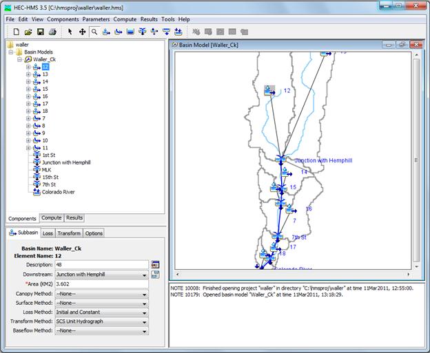
After this icon is highlighted, the Parameters panel show the information related to this Sub-basin. In the first tab (Sub-basin Tab) you will find the the area of sub-basin 12 (3.602 sq. km). Make a note of this value. Go ahead and look up the areas of the other sub-basins as well. HMS can work with a Basin file in either SI or English units. In this case, the file is in SI units.
To be turned in: a table showing the areas of the subbasins. What is the total drainage area of Waller Creek (sq. km)?
Returning to the HMS, focus your attention on the icons over the Top Menu. The ![]() button allows you to select (highlight) items in the model. You may also use
the
button allows you to select (highlight) items in the model. You may also use
the ![]() button to drag-and-drop hydrologic elements from the left-hand-side of the
window or to move individual elements within the model. If you have a model
element highlighted, you can view its properties in the Parameters Panel on the lower left hand side of the display.
The
button to drag-and-drop hydrologic elements from the left-hand-side of the
window or to move individual elements within the model. If you have a model
element highlighted, you can view its properties in the Parameters Panel on the lower left hand side of the display.
The ![]() button allows you to move (or pan) the entire model display by holding down the
left mouse button and moving the mouse. If you wish to zoom in or out, you may
do so by depressing the
button allows you to move (or pan) the entire model display by holding down the
left mouse button and moving the mouse. If you wish to zoom in or out, you may
do so by depressing the ![]() button, left click and hold to select a rectangle area in Basin Model to zoom
in, to zoom out just right click in the window. Go ahead and experiment with
these buttons to understand better how each works. I had some trouble making the Pan tool to
work.
button, left click and hold to select a rectangle area in Basin Model to zoom
in, to zoom out just right click in the window. Go ahead and experiment with
these buttons to understand better how each works. I had some trouble making the Pan tool to
work.
In the Top Menu under View we have the following options checked:
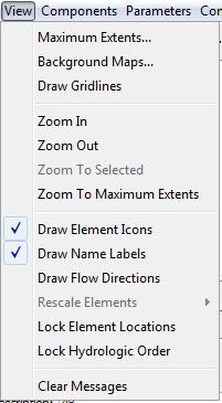
Click in Draw Flow Direction to
check this option too, now the reaches will show the flow direction with the
symbol ![]() .
If you Uncheck the Draw Element Icons you will see only the text name of the hydrologic
elements, in the next figure you can see this, in the left side the Draw
Elements Icons is checked and in the right side is unchecked
.
If you Uncheck the Draw Element Icons you will see only the text name of the hydrologic
elements, in the next figure you can see this, in the left side the Draw
Elements Icons is checked and in the right side is unchecked
 .
.
As needed, you may create new
hydrologic elements in the model area, to do this just click in one of the
icons ![]() and then click in an empty space in the Basin
Model Panel (after doing this the program will ask for a name and
description for the new element, give those and press create). Go ahead and try
this, but make sure you keep the elements you add away from the elements
currently in the model. Try taking a river reach and connecting a junction to
each end. To do this, create one
and then click in an empty space in the Basin
Model Panel (after doing this the program will ask for a name and
description for the new element, give those and press create). Go ahead and try
this, but make sure you keep the elements you add away from the elements
currently in the model. Try taking a river reach and connecting a junction to
each end. To do this, create one ![]() and two
and two ![]() junctions. Hook up one end of the river reach to one junction by drag-and-drop
the river reach end to the junction (use
junctions. Hook up one end of the river reach to one junction by drag-and-drop
the river reach end to the junction (use ![]() ).
If you do it correctly drag-and-drop the junction in another part of the map
and the river reach end will follow the movement to the new place because they
are hooked. Repeat these steps appropriately to connect the stream to the other
junction. To delete the elements you have added when you are finished,
highlight all added elements (hold down the shift key to keep adding elements)
and then right click in one of them and choose Delete Elements. If you
want, take some time now to experiment with some of the other hydrologic
elements.
).
If you do it correctly drag-and-drop the junction in another part of the map
and the river reach end will follow the movement to the new place because they
are hooked. Repeat these steps appropriately to connect the stream to the other
junction. To delete the elements you have added when you are finished,
highlight all added elements (hold down the shift key to keep adding elements)
and then right click in one of them and choose Delete Elements. If you
want, take some time now to experiment with some of the other hydrologic
elements.
As the calculation steps above suggest, the primary function of a surface-water model such as the HMS involves three sets of calculations--quantifying rainfall losses into the soil, converting excess rainfall to runoff, and routing. As part of creating a HMS model, the selection of the processes to be used for each calculation set is made in the Parameters Option in the Top Menu.

First Select Parameters/Loss/Initial and Constant, the Initial and Constant method is the only option available because is the method selected (if we want to change the method we can do it selecting Change Method… at the end of the list, and select one of the others methods listed)
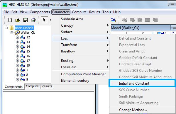
The following window should appear in the place of the Basin Model Panel.
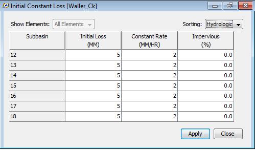
Note that the Initial/Constant Loss Rate parameters are entered is in this table. Each basin requires an initial loss quantity, a constant loss rate, and a percent imperviousness. These values have been selected arbitrarily. If the % impervious value differs from 0, that % of the land area is assumed to have no losses and the loss method is applied only to the remainder of the drainage area
After you have looked over the data, click Close. For future reference, while both Close and Apply transfer the data to the computer's short-term memory, they differ only in that Close closes the window while Apply keeps the window open.
Once you have closed the Initial/Constant Loss window, choose Parameters/Transform/SCS:
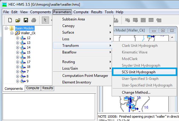
Similar to Parameters/Loss, in this section the only option available is SCS Unit hydrograph method (also if we want to change the method we can do it selecting Change Method… at the end of the list, and select one of the others methods listed), click in SCS Unit Hydrograph will display the following window.

Note that the SCS unit hydrograph method requires only one parameter for each sub-basin--lag time between rainfall and runoff in the subbasin. HMS. At this point, go ahead and close this window.
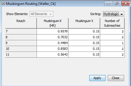
The next step involves entering the parameters for the routing process. From Parameters/ Reach / Muskingum.
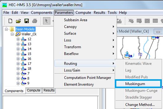
This should cause the following image to appear. This simulation routes the water through the reaches by the Muskingum method in which K is the travel time of a flood wave passing through the reach, X is a measure of the degree of storage (X = 0 means a level-pool reservoir or maximum storage, X = 0.5 means a pure transmission reach in which there are no storage effects, and X ranges between 0 and 0.5). The reach is divided into a number of subreaches if necessary to keep the computations numerically stable.
You do not have to go through the Parameters menu to edit element properties. Editing may also be accomplished by highlighting an element, and changing the options in the Parameters Panel.
In the Parameters/Baseflow option of the HMS, you supply if necessary, information such as basin areas and initial base flows in the system. In this model we are not allowing for any base flow
To be turned in: Select subwatershed 14 and reach 10 and describe in words what the parameter values are that are used to characterize these hydrologic features.
3. Creating a Precipitation Model
Having established the physical aspects of the model, we will now address
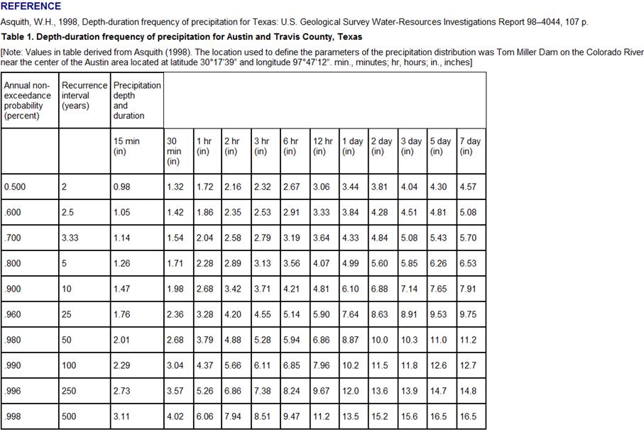
the rainfall data. From a statistical study of extreme storm rainfall
data recorded at gages, tables and maps have been prepared for the whole US
which specify the storm precipitation depth to be expected as a function of the
return period of the event and the duration of the rainfall. A table of
such values is shown below for
http://www.amlegal.com/austin_nxt2/gateway.dll?f=templates&fn=default.htm&vid=amlegal:austin_drainage
![]() We are going to input
the rainfall to HM. To create a design precipitation input file, go to the
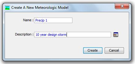
Project Window and select Component/ Meteorologic Model Manager/New. A window like
this appears in which you can describe the precipitation file you intend to
create, in this case for a 10 year storm.
We are going to input
the rainfall to HM. To create a design precipitation input file, go to the
Project Window and select Component/ Meteorologic Model Manager/New. A window like
this appears in which you can describe the precipitation file you intend to
create, in this case for a 10 year storm.
![]()
![]()

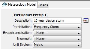
Write Precip 1 as name and 10 year design storm in description, then click create.
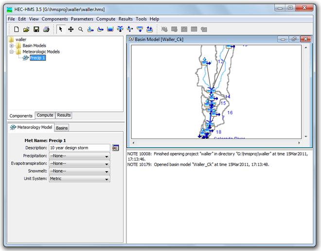
After clicking, create, close the Meteorologic Model Manager; in the Main Window, the Data Panel will display a Metereologic Models Folder which contains the Precip 1 model created in the previous step, select this Model.
In the Precipitation combo box select Frequency Storm
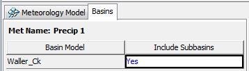
Select Basins tab and for the Waller_Ck Basin Model change the Include Subbasins options to yes.
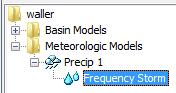
In the Data Panel, expand the options for Precip 1 and select Frequency Storm
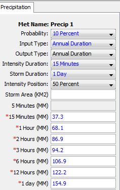
Now, in the Parameters panel fill in the values shown from the table above for a 10 year storm (10% chance of being equaled or exceeded in any year), as input type select Annual Duration, for Intensity Duration select 15 minutes, for Storm Duration select 1 Day don’t forget to use the correct precipitation units! (The program will ask you for millimeters). Here are the data for the 10 year return period storm:
|
Duration |
15min |
30min |
1 hr |
2 hr |
3 hr |
6 hr |
12 hr |
1 day |
|
Depth
(inches) |
1.47 |
1.98 |
2.68 |
3.42 |
3.71 |
4.21 |
4.81 |
6.10 |
|
Depth
(mm) |
37.3 |
50.3 |
68.1 |
86.9 |
94.2 |
106.9 |
122.2 |
154.9 |
For each project, the HMS then creates an output Data Storage System DSS file which stores calculated data from all runs for a given project so that results from a previous run can be directly compared to results from a more current run.
To be turned in: a screen capture of the design precipitation input file
4. Defining the
Control Specifications
The final piece of the model setup involves establishing the model's time limits. Go back to the Top Menu and select Parameters/Control Specifications Manager/New.
![]()
![]()
![]()
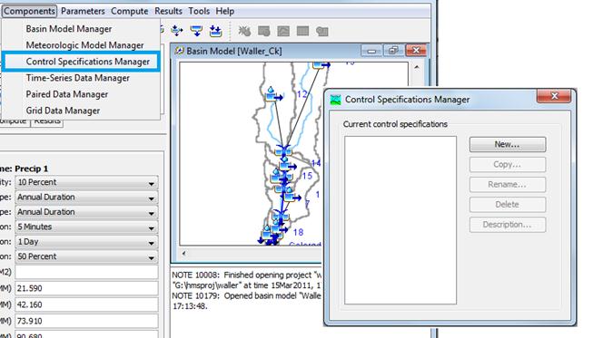
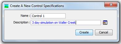
The following window will appear in which you can label the name and description.
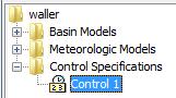
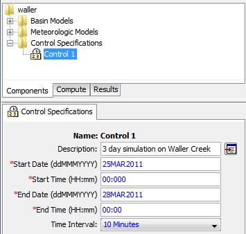
Click Create and close the Control Specifications Manager, in the Data Panel, expand the options for Control Specifications and select Control 1
In the Parameter Panel, specify the duration of the simulation in date and time, and also the time interval of the calculations (10 minutes). In this case, the duration is arbitrary, long enough to depict the runoff from a 1-day storm, but the 10 minute time interval is part of the Basin file model setup and should remain fixed for this Waller Creek model.
To be turned in: how many time intervals of computation will be performed?
5.
Executing an HMS Model
Finally, you have finished perusing the data involved in creating the Tenkiller model. In the Top Menu select Compute/Create Simulation Run.

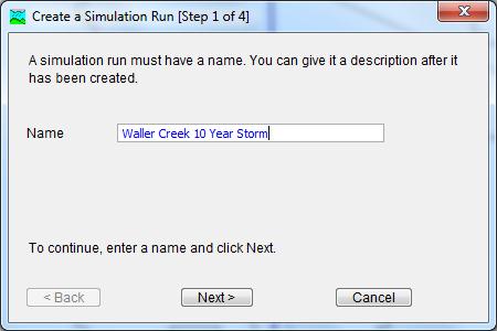
In the following four steps the simulation will be created,
in the first step specify the Name of the Simulation 10 years Waller Creek and click
next >
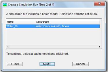
In the second step we select the Basin Model Waller_Ck (the
only one that we have) and click next
>
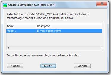
The third step corresponds to the Meteorological model, select Precip 1 and press next >
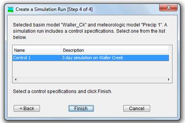
Finally, in the fourth step we select the Control 1 of the Control Specifications and click finish.
After completing the previous steps, the simulation is created (although we need to run it), you can see it in the Data Panel, in the Compute tab

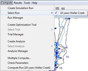
In the Main Window, select Compute/Select Run and you will see that 10 years Waller Creek is checked; in the case of multiple simulations runs it is important to check (select) the one that we want.
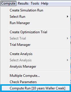
To run the model, go the Top Menu and Compute/Compute Run [Waller Creek 10 Year Storm]
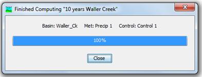
You should get a window that says the following:
If you want to make runs with alternative model files, you
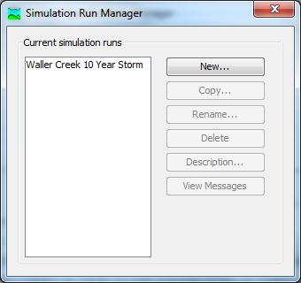
Create different simulations runs in the Top Menu select Compute/Create Simulation Run (and follow the four steps described previously), check the simulation in Compute/Select Run and Compute/Compute Run [Name of the new simulation], the HMS allows the user to have multiple data sets available to include conveniently in different runs.
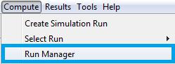
Choose Compute / Run Manager. You should see an image similar to this: which shows what files were used on this Run.
6.
Viewing HMS Results
The HMS allows you to view results in tabular or graphical form. To view a global results table, in the Top Menu select Results/Global Summary Table. I had trouble getting this to work properly.
You may view results for each element within the model. To do this, in the Data Panel Select Results expand Waller Creek 10 Year Storm and also the Junction 15th St and select graph, you should see the following:
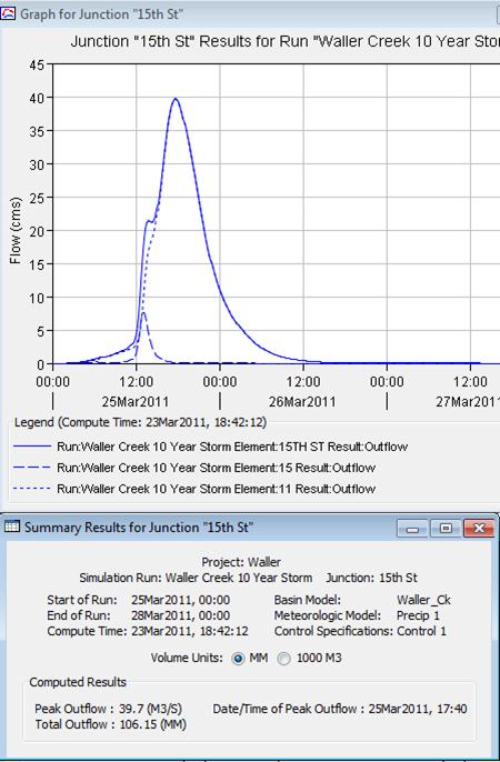
To be turned in: Make a table showing the peak discharge in cms at each of the six outlet points on Waller Creek (5 junctions and 1 sink).. What is the drainage area above each of these points? What is the peak discharge per unit of drainage area (cms/sq. km) for these points?
Waller Creek Diversion Design
Study
The citizens of Austin approved a bond issue which authorized
the City to borrow funds for the construction of a flood diversion tunnel for Waller
Creek. http://www.ci.austin.tx.us/wallercreek/wctp_home.htm
At present, the
100 year flood plain for the creek covers many city blocks in downtown
Austin. The goal is to make this area safer from floods and also to
encourage the development of a river walk area, perhaps similar to that in
Recompute the flows from the HMS model using the
100 year design storm instead of the 10 year design storm. How much water would have to be diverted at
Recompute the flows from the HMS model using a
2-year, 5-year, 25-year, and 50-year storms.
Make a plot showing the peak discharge to be expected from these events
at
To be turned in: A graph and a table showing the
relationship between flood peak discharge and return period for Waller Creek at
15th St. Determine the flow
diversion needed at
Summary of Items to
be Turned In:
(1) a table showing the areas of the subbasins. What is the total drainage area of Waller Creek (sq. km)?
(2) Select subwatershed 14 and reach 10 and describe in words what the parameter values are that are used to characterize these hydrologic features.
(3) a screen capture of the design precipitation input file
(4) how many time intervals of computation will be performed?
(5) make a table showing the peak discharge in cms at each of the six outlet points on Waller Creek (5 junctions and 1 sink).. What is the drainage area above each of these points? What is the peak discharge per unit of drainage area (cms/sq. km) for these points?
(6) a graph and a table showing the relationship
between flood peak discharge and return period for Waller Creek at 15th
St. Determine the flow diversion needed
at