Exercise 5a. Nutrient Load Calculation of San Marcos Basin
GIS in Water Resources
Fall 2010
Prepared by Tony Castronova, Jingqi Dong
Computer and Data Requirements
Loading Data into HydroDesktop
Loading the HydroModeler Extension
Creating Links Between Model Components
The HydroModeler is a modeling extension of HydroDesktop that adds the capability for a user to process data that was harvested using the HydroDesktop search mechanism. This exercise will show you how to construct a model using the HydroModeler, process data, and reload the results back into HydroDesktop to visualize them. To illustrate the usage of this extension a model will be constructed to calculate the nitrogen loading at two gauge stations within the San Marcos basin. The model will consist of several HydroModeler components that have been previously developed, and will be driven by nitrogen concentration and streamflow measurements.
Version 1.1 Beta 294 (Fri Oct 22 2010) or later of HydroDesktop must be installed on the computer. It is available at www.HydroDesktop.org.
Logon to the computer of your choice and make a directory in your workspace for this exercise. The required files can be downloaded from the class website. Use Windows Explorer to create a folder called Ex5 and within this location create a folder called Data. Unzip “HydroModelerData.zip” in this folder.
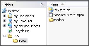
You should see a file called SanMarcosData.sqlite. This database contains streamflow and total nitrogen concentration at one USGS gauge location within the San Marcos basin, named San Marcos Rv at Luling, TX. This was downloaded for you using the HydroDesktop search feature. You will also see a folder called models. This folder contains some model components that will be used to perform a nitrogen loading calculation.
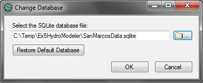
Launch HydroDesktop. In order to use the data stored in the SanMarcosData.sqlite database, it must first be loaded into HydroDesktop. To do this, select the Table ribbon tab and under the Database category, click the Change button.
A new window will appear. Navigate to the path where the SanMarcosData.sqlite was saved and click OK.
You should now see 2 data series (see below).

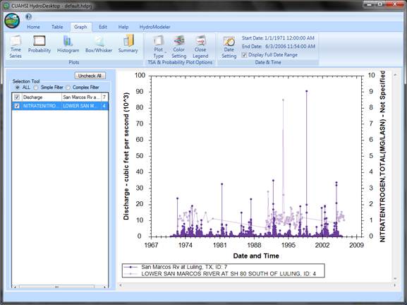
The actual values of these data series can be visualized by selecting the Graph ribbon tab. Check the boxes next to the Flow rate and Total nitrogen quantities for each site id. You can see that data is available at each site, although not always at the same time. Keep patient when Discharge data is loading.
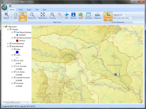
Navigate back to the Home ribbon tab to spatially visualize this data. Here we can see where the gauge exists in the San Marcos basin. Using the Basemap tool learned in Exercise 1, you can get the following fancy map showing the actual location of San Marcos Rv at Luling, TX.
![]()
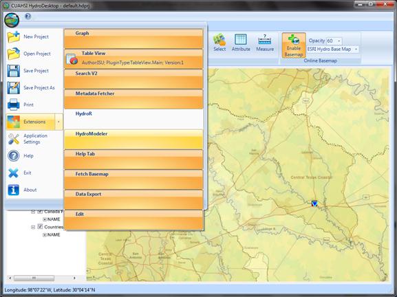
HydroModeler is an extension for HydroDesktop that provides a hydrologic modeling environment. This will be used to perform a nutrient loading calculation at the selected site, but only when both “Flow rate” and “Total nitrogen” exist at the same time. To do this, the HydroModeler extension must first be added by clicking on the Orb located in the top left corner of the HydroDesktop application, then selecting Extensions, and finally selecting HydroModeler.
The HydroModeler extension will automatically launch and you should see something like this (see below). There are three main components to HydroModeler: File Browser window, Properties window, and Composition window. The File Browser window is used to navigate and find “model components”. These “model components” are individual computations that can be loaded into the Composition window to form a “model composition”. The Properties window is used to display and modify the properties of a “model component” that is selected in the File Browser window.
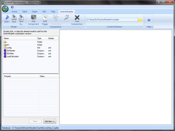
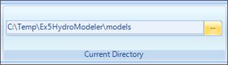
Navigate to the folder where you saved the exercise data and then into the models folder. You can do this using the File Browser window or by changing path in the Current Directory textbox.
Next, you should see a file named DbReader in the File Browser window. This is a model component designed to read data from the HydroDesktop database. Click once on the DbReader component to populate its attributes in the Properties window.

The values listed in the Properties window can tell us a little about the DbReader model component such as its class name, where the assembly is located, and an argument called RangeInSeconds. This argument allows the modeler to specify a search window to look for data. For instance, the current value of 86400 states that the DbReader will search for data within a 24 hour time window of all requested times. This is helpful if calculations are being performed on two different data series having different (or inconsistent) measurement intervals. Of course, there remains the possibility that more than one data value is found within the specified search window. In this case, the DbReader will average all of the values it finds. Since the stream flow data series contains daily recorded data and the nitrogen series contains values recorded every ~15 days, we must choose an appropriate RangeInSeconds as to not waste computational time. Click on 86400 and change its value to 2592000 (30 days), press Enter and then select Save. Next load the DbReader component by simply dragging it from the FileBrowser and dropping it into the Composition window.


Next, add the DbWriter component to the Composition Window. This component is responsible for extracting time series data from the HydroModeler and saving it in the HydroDesktop database. The IgnoreValue argument, shown in the properties window, allows the modeler to specify which (if any) value will be ignored and thereby NOT saved to the database. For now, leave this as -1.
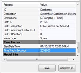
Next, locate the LoadCalculator. Click on the LoadCalculator model component once to see its attributes in the Properties window. You should see various arguments that describe the model. These arguments can be modified to resemble the desired study area. Scroll all the way to the way down and change TimeStepInSeconds to 2592000. Next, we need to adjust this component’s start time by changing StartDateTime to 01/15/1975 12:00:00.
Finally, Save these changes and add the LoadCalculator component to the model composition.
Lastly, add a Trigger to the composition by clicking the Add Trigger ribbon button at the top of the screen.

Now we have all the necessary model components to read the data from the database, perform a load calculation on the data, and then write the data back into the database. The Trigger is a mechanism that defines the end of the model, and is used behind-the-scenes to moderate the simulation run.
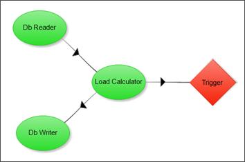
The next thing to do is create connections between the individual model components. These connections represent the pathways for data to flow between components. To add a link, click the Add Connection ribbon button then click the desired “source” model component followed by the desired “target” model component. For example, to create a linkage between the DbReader and LoadCalculator, click the DbReader component then the LoadCalculator component.
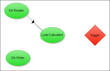
Repeat this to draw links from the LoadCalculator to the DbWriter, and the LoadCalculator to the Trigger. The model composition should look like this.
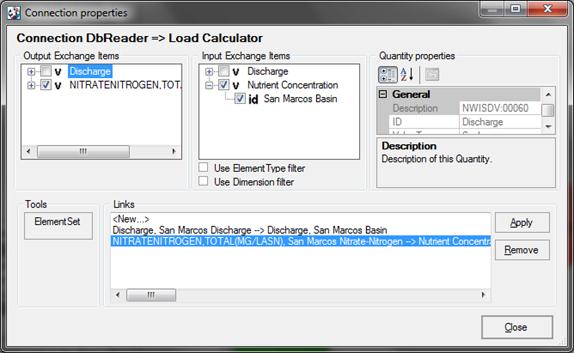
Next, we need to define the data that will travel across each link. Click on the Arrow between the DbReader and LoadCalculator, you should see the following window.

Click on the plus sign next to the Discharge item and check the box next the San Marcos Discharge. Then click the plus sign next to Discharge and check the box next to San Marcos Basin. Finally click the Apply button. This action tells HydroModeler that the “Flow rate” from the DbReader will be supplied as “Discharge” to the LoadCalculator during the simulation. Repeat this to define a linkage between NitrateNitrogen,Total and Nutrient Concentration as well.
NOTE: Be patient as this step may take a few extra seconds to complete.
Close this window and repeat these steps for the link between the LoadCalculator and DbWriter, only this time choose Nutrient Load and any quantity.

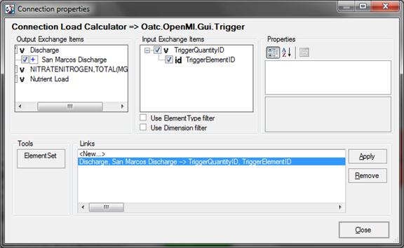
Finally, click the link between the LoadCalculator and the Trigger. Specify Discharge and San Marcus Discharge to TriggerQuantityID and TiggerElementID.
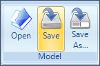
Save the model composition by clicking the Save ribbon button.
Click the Run ribbon button to open the “Run properties” dialog.
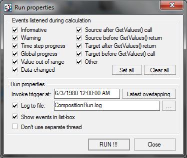
Click the Set all button to turn all model notifications on. HydroModeler will automatically select the end time by based on the time horizons of all the components if “Latest overlapping” is clicked. Since model the entire series of data will take a significant amount of time, we can instead manually specify the model end time by changing Invoke Trigger At to 6/3/1980 12:00:00 AM. Finally select RUN !!! Model simulation should about 3 minutes. When it’s finished the dialog box should look like this.

Close this window, and select Yes at the next dialog window to reload the model components.
NOTE: Be patient as this step will take a few extra seconds to complete because each model will be reloaded.
To view simulation results, first select the Table ribbon tab and click the Refresh button. You should see one new data series labeled Nutrient Load.
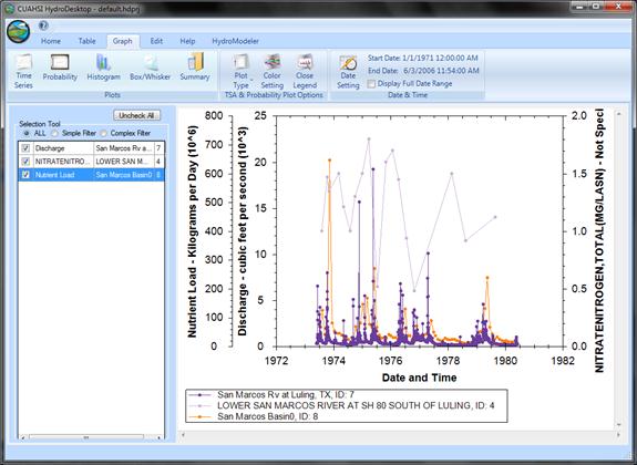
To view the series values, click the Graph ribbon tab and choose the desired series.
Here are the streamflow (dark purple line), nitrate-nitrogen concentration (light purple), and the nitrogen loading (orange line) for San Marcos Rv at Luling, TX all on a single plot. You can select Date Setting option to specify the date range so that only data during the dates that were simulated are shown in the plot.
Here is the exported graph of nitrogen loading that was calculated.
That’s the end of our procedure. You have successfully performed a simple nitrogen loading calculation. This model can be adjusted to fit different data by modifying the DbReader’s RangeInSeconds argument and/or the LoadCalculator’s TimeStepInSeconds argument.