Image Analysis
and Classification Techniques using ArcGIS 10
Prepared
by Pari Ranade and Ayse Irmak
GIS in
Water Resources
Fall 2010
Purpose
The
purpose of this exercise is to perform typical tasks of remote sensing analysis
using ArcGIS 10. We will perform georeferencing, image interpretation and image
classification. We will use Google captured image as an example for
georeferencing. Landsat 5 image for image interpretationa and image
classification. With this exercise you will –
1.
Capture image from Google for Lincoln are and Georeference it.
2.
Perform Image analysis and identify features in the Landsat 5 images of July
and Feb for Lancaster County. (display false and true color composites)
3.
Compute NDVI
4.
Could mask the image
5.
Perform supervised and unsupervised classification
6.
Compare classified map with existing NASS and CALMIT landuse
Computer
and Data Requirements
To carry out this exercise, you
need to have a computer, which runs the ArcInfo
version of ArcGIS 10. There is no need for remote sensing software. The data
are provided in the accompanying zip file, http://www.caee.utexas.edu/prof/maidment/giswr2010/Ex6/Ex6.zip
Downloading
Landsat data
Landsat data can be
downloaded for free from http://edcsns17.cr.usgs.gov/EarthExplorer/ or http://glovis.usgs.gov/. USGS global visualization
viewer facilitates viewing and downloading of satellite imagery. USGS provides
Landsat 5 TM data in TIFF format.
This data can be converted into other formats using ArcGIS or any image
processing software (i.e. ERDAS-IMAGINE,
ENVI). Landsat satellite passes over earth, the area can be identified by
the path and row combination. Our study area is under the path 28 row 32. This
is southeastern part of Nebraska and Landsat passes over this area at
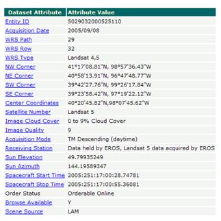
approximately 10:15 CST. Each Landsat scene has a unique identifier. Our
dataset has identifier LT50290322005251EDC00. All the information regarding
Landsat data can be found in Header file of Landsat data. These files will end with _GCP and _MTL.
These files also contain the information regarding each band pertinent to that
scene. Useful information like center and corner coordinates of Landsat scene
is also provided in the header file. A screen shot of sample attributes for
this Landsat scene is provided below.
Landsat 5 TM has 7
different bands. These bands are useful for extracting various information
related to vegetation, temperature, clouds, soil moisture, biomass, rocks,
minerals and so on. Below are details of
band designation for Landsat 5 TM. More detailed information can be found at http://egsc.usgs.gov/isb/pubs/factsheets/fs02303.html.
|
Band |
Spectral
Bands1 |
Wavelength
(micrometers) |
Potential
Information Content |
Resolution
(meters) |
|
Band 1 |
Blue |
0.45 - 0.52 |
Discriminates
soil and rock surfaces from vegetation. Provides increased penetration of
water bodies |
30 |
|
Band 2 |
Green |
0.52 - 0.60 |
Useful for
assessing plant vigor |
30 |
|
Band 3 |
Red |
0.63 - 0.69 |
Discriminates
vegetation slopes |
30 |
|
Band 4 |
Near IR |
0.76 - 0.90 |
Biomass content
and shorelines |
30 |
|
Band 5 |
Mid
IR |
1.55 - 1.75 |
Discriminates
moisture content of soil and vegetation; penetrates thin clouds. |
30 |
|
Band 6 |
Thermal IR |
10.40 - 12.50 |
thermal mapping
and estimated soil moisture |
120 |
|
Band 7 |
Mid
IR |
2.08 - 2.35 |
Mapping
hydrothermally altered rocks associated with mineral deposits |
30 |
1: IR
stands for infrared
Various composites
can be mapped to facilitate viewing of the raw imagery. A false color composite of near infrared is useful for observing
spatial distribution of the vegetation in the Landsat scene by combining bands 2, 3 & 4 (RGB). We are going to generate
the true color composite by using
spectral bands 2 (green), 3 (red), and 4 (near infrared).
Part I –
Georeferencing
Raster data or
imagery served by various agencies usually has spatial reference. However
sometimes the location information delivered with them is inadequate and the
data does not align properly with other data you may have. Sometimes raster
data is digitized using scanned paper maps and co-ordinate system needs to be
assigned. Thus, to use some raster
datasets in conjunction with your other spatial data, you may need to align, or
georeference, to a map coordinate system. Georeferencing raster data allows it to be
viewed, queried, and analyzed with other geographic data.
In this exercise,
we will use Google map to as a source raw image to be georeferenced. With
ArcMap 10 we can use Bing maps directly in ArcMap as basemaps. But google map
is just an illustration of how we can use our own map and add spatial reference
to it. The mapped could be scanned image of your field map or any other scanned
hard copy map.
Go to http://maps.google.com/. Search for Lincoln, NE. Click on the Satellite
option on upper right corner of google map. On the Northwest
side of the map you will see Capitol
Beach Lake near I-80. Interstate
80 is a major transcontinental corridor connecting California and New York
City.
Go to New! On upper right corner of the
webpage. Enable LatLng Marker. This will
enable to mark the longitude and latitudes of the locations of the map. You can
also enable LatLng Tooptip as well
if you wish. Right click on the
point where you need to mark the lat-long select drop latlng option. To zoom in the specific are using right click and select zoom in option. It is handy compared to
zoom in bar on the Google.
Raster is georeferenced
using existing spatial data (target data),
such as a vector feature class, that resides in the desired map coordinate
system. The process involves identifying a series of ground control points—known x,y coordinates—that link
locations on the raster dataset with locations in the spatially referenced data
(target data). Control points are locations that can be accurately identified on
the raster dataset and in real-world coordinates. There are many different
types of features that can be used as identifiable locations, such as road or stream intersections, the mouth of
a stream, rocky outcrops, the end of a jetty of land, the corner of an
established field, street corners, or the intersection of two hedgerows.
Similar to shown in
figure, try to identify the control points which are unique and easy to locate
on the map. Try to avoid control points
which are too close to each other. Also try to find control points from all regions of the image. Capture the screen
using PrintScreen button on keyboard
and paste it in Paint and save it as an image. Paint can be opened on windows
PC from Start/Programs/Accessories/Paint.
Note down the Latitude and longitude
information for each control point
and save the image as ControlPts.TIF.
This will be your reference if you note the control points incorrectly.

Close the LatLng Tooltip and uncheck the Show lables option under
satellite. Again capture the screen,
open the paint and paste the image. Crop the image to clean the sides of the
image. You have been provided with Lancaster
county feature class, NASS and CALMIT land use maps for comparison after we
georeference the Google captured image. Entire data is under Lancaster Geodatabse in Ex6 folder. Go to ArcCatalog and under
the Ex 6 folder create and new personal
geodatabase name it as EX6. Save the image as TIFF format with name Capitol
Beach under EX6 personal
geodatabase. Add the Capitol Beach.TIF to
ArcMap. Now you will see clear satellite image of Capitol Beach without any
labels or location information.
Open ArcMap and set
the coordinate system of the frame for proper alignment. Right click on layers![]() . Go to Properties\coordinate system/import.
Select the Lancaster_County polygon
in Lancaster geodatabase.
. Go to Properties\coordinate system/import.
Select the Lancaster_County polygon
in Lancaster geodatabase.
Now we have
identified the control points with Lat Long information, we will import them in
ArcGIS. Open ArcCatalog. Right click on Ex6 geogatabase, select new/feature class. Name it as Control_Points alias Control_Points . Select point feature
type. Select the Spatial reference in
Geographic Coordinate System/World/WGS
1984.prj. Leave rest of the options as default. This is the coordinate system that Google
uses.
Go
to Toolbars/Editor to open editor
toolbar.
Start
Editing the Control_Points. Open the Capitol Beach.TIF that you have saved
under Ex6 geodatabse. You might receive warning about unknown spatial reference. Click OK.

In create feature window choose create control points layer and under construction tools choose point. Right click on any point within
layer and select Absolute X,Y…Type X (lat) and Y (Long) that you have recorded from Google LatLng marker for each control point.
Complete the same
procedure for all the control points that you have selected. If you enter the wrong LatLong information, you can delete the point and add it again. Stop editing and save
your edits. Now you have completed the control points feature layer. This was
to illustrate one way of adding control points. Another simpler way is to add control points using Make XY event layer tools from text or excel table. Tool is located
under data management\layers and table
views. You will later export this layer as point feature class with the name Control_Points in Ex6
geodatabase.
Now we will start
georeferencing the Capitol Beach.TIF. Go
to customize/toolbars/georeferencing. Make sure Capitol beach layer is selected for georeferencing. Click on add control points ![]() button.
button.
This button will
link our Control_Point features to
the same location on the Capitol
Beach.TIF, Which means we will kind of assign spatial reference to the control points on Capitol Beach.TIF. ArcGIS then will fit the surface and assign
spatial reference to entire image.
Now let’s start
adding the control points![]() . Make
sure you Auto Adjust option is on
both on Georeferencing toolbar and
on Link table. Link table can be
opened by clicking on
. Make
sure you Auto Adjust option is on
both on Georeferencing toolbar and
on Link table. Link table can be
opened by clicking on ![]() button on Georeferencing toolbar.
button on Georeferencing toolbar.
You might not be
able to see anything in full extent since, on Capitol Beach.TIF is missing a spatial reference. Right click on Capitol Beach.TIF layer click on Zoom to Layer. Now identify the location of one of control point on the image and click on
the location on image. Here you can refer to your ControlPts.TIF image where you have saved the LatLong information of each control point on image.
Now right click on
the Control_Point layer and ‘Zoom to Layer’ (your cursor will be
showing line, disregards that). Now you will see all the control points. Click
on the control point which corresponds to point on the image, now ArcGIS snapping environment will be
automatically activated and your control point will be snapped. Notice your
both layers are now closer. Continue adding the control points. You might
receive the warning that ‘The control
points are collinear or not well distributed, this will affect the warp result’
Click OK and see how much of warping
(shift) is caused. If you think image is warped too much, it indicates you have
misplaced the control point.
If you misplace a
control point, simply click on the view link table button ![]() and delete the control point (selected
control point will be in highlighted in blue as shown in figure). Notice once
you have added the second control point you Capitol Beach.TIF and Control_Point layers will be aligned. This is
due to Auto adjust function. Now
finish all the control points.
and delete the control point (selected
control point will be in highlighted in blue as shown in figure). Notice once
you have added the second control point you Capitol Beach.TIF and Control_Point layers will be aligned. This is
due to Auto adjust function. Now
finish all the control points.
Open the View link table![]() . Make
sure Auto adjust option is checked.
Compare the transformation options – 1st
order polynomial (affine), 2nd order polynomial and adjust. See
which image looks most similar to your original image from Google. Select the
best fitted transformation and click OK.
. Make
sure Auto adjust option is checked.
Compare the transformation options – 1st
order polynomial (affine), 2nd order polynomial and adjust. See
which image looks most similar to your original image from Google. Select the
best fitted transformation and click OK.
Q.
Turn in the image with all three Transformation option. Label the image to show
which transformation is used.
Click on the Update georeferencing option under
georeferencing toolbar. Next click on the Rectify
option on georeferencing toolbar.
Change the Name of the file to ‘Captiol_Beach_Rect’
and Output location to Ex6 geodatabase.
Leave rest of the option to default and click SAVE.

Remove Control_Points layers and Capitol_Beach layer from ArcMap. Open
the ArcCatalog. Right click on the Captiol_Beach_Rect
image from Ex6 geodatabse that you
have just saved. (Note: sometime you might have to reopen the ArcCatalog if it
was already open, or refresh it from View/refresh or use F5 key on keyboard).
Notice your file now has a spatial reference GCS_WGS_1984 and datum D_WGS_1984, which is same as Google data.
Open Captiol_Beach_Rect image in ArcCatalog
from Ex6 geodatabse. Now we need to reproject it in the Nebraska State
Plain coordinate system (NAD 1983
StatePlane Nebraska FIPS 2600 Feet) in which all the Lancaster county data is.
Search for Project raster under tools in ArcGIS.
It is located under Data management
tools/projections and transformations/raster/project raster. Save the
output raster data with the name ‘Captiol_Beach_Rect_Proj.img’
under Ex6 geodatabase. Click on the
output coordinate system and import from CALMIT_2005
layer from Lancaster geodatabase. Now it should show as ‘NAD_1983_StatePlane_Nebraska_FIPS_2600_Feet’. Select the Geographic transformation as ‘WGS_1984_(ITRF00)_To_NAD_1983’Leave the
rest of the options to default.
‘Captiol_Beach_Rect_Proj’ layer will be
added after the tool has run. Wait till it runs completely and you receive
successful message. Remove the ‘Captiol_Beach_Rect’ layer from the ArcMap.
(Make sure your the coordinate system of the frame is Nebraska State Plane. Else
right click on layers![]() . Go to Properties\coordinate system/import.
Select the Lancaster_County polygon
in Lancaster geodatabase. )
. Go to Properties\coordinate system/import.
Select the Lancaster_County polygon
in Lancaster geodatabase. )
Add
‘Lancaster_County’, ‘CALMIT_2005’ and
‘NASS_2005’ layers from Lancaster geodatabase. Change symbology of ‘Lancaster_County’ to ESRI hollow. Bring the ‘Captiol_Beach_Rect_Proj’ layer on top.
Make sure ‘CALMIT_2005’ layer is
just below that. Zoom in to the ‘Captiol_Beach_Rect_Proj’
layer .
Right click on the ‘Captiol_Beach_Rect_Proj’
layer and go to properties/display,
set transpaancy to 30%. Observe the symbology of the ‘CALMIT_2005’ layer for ‘roads’ (most
probably black). See how Interstate – 80 is aligned with the Roads in
‘CALMIT_2005’ layer. This is indication that you have correctly georeferenced
the TIF file.
Q
Turn in the image showing overlay of CALMIT landuse and rectified Google image
(30% transparent). What land uses are present on the Northwest side of the
I-80. Which waterbody is present on the North west side of the I-80? What is
another indication of presence of water body (which land use)?
Part
II – Image interpretation
We can utilize the
Image Analysis window to visualize and analyze the imagery. These tools will
enhance the imagery in order to better interpret the imagery. Go to Window/Image Analysis. Now image
analysis window will open. Select the layers that you want to work with. Note
that layer shown in a blue is the one which you are working currently. Simply
checking the box won’t make the tools work on layer.
We can use
different band combinations of RGB to interpret the images. We can interpret
various features in the imagery such as vegetation, buildings, streets, water
bodies, landmarks structures. I want to look at different kinds of vegetation.
We can even work with historical imagery-you know temporal information.
Open July and Feb
images from the Lancaster Geodatabse. Change RGB layers to 3, 2, 1 respectively. You
need to left mouse click on the rectangle (each for red, green, and blue) and
assign the layer to it. This is called a
natural-color composite where image features will be visible in natural
color. Also open the georectified image of capitol Beach. On the Northwest side of the georectified
image you will see a structure just opposite the road (I-80). This is Lincoln
municipal airport. Now we will use Display tools in image analysis window to
enhance the image. Select Feb image and change display option – 1. Gamma – 0.50
and check DRA. Leave rest of the options to default. You will notice the now
that image features such as capitol beach in blue color, airport buildings in
white colors and soil in brownish color. Features are more identifiable after
enhancement. Remember these changes are
not permanent and you need to take a screen shot while you are performing the
exercise.
Q Turn in the picture of Lincoln Municipal Airport in February
before and after enhancement using display tools
Now
lets see what these tools are doing. Gamma tool will adjust the mid level
values without bleaching out the image. So this leaves the black and the white,
more of those values alone will adjust into mid values like you see here. One
thing I can do is change the stretching function. So you see there are several
I can choose from. DRA is called dynamic range adjustment and it dynamically
adjusting the display of the image based on the pixel values that are currently
visible. So it only optimizes the values that are currently on your screen. You can explore other tools by playing around
them. It would not make changes to original image.
Now
change remove the Feb and July images and add them again to ArcMap. Now change
the RGB combination to 4, 3, 2. This is called a false-color composite. It will
enhance the vegetation in the image. Try to enhance the image if you need to.
These
tool can be used to compare the images - zoom to raster resolution![]() , swipe
layer
, swipe
layer![]() , flicker
layer
, flicker
layer![]() buttons.
Explore these buttons. Note swipe layer button brigs special arrow, so hold on
left mouse click, drag it across the images.
buttons.
Explore these buttons. Note swipe layer button brigs special arrow, so hold on
left mouse click, drag it across the images.
Q. What is the prominent
difference between July and Feb images of the Lincoln Municipal Airport with
false color composite?
Now we
will use some of the Processing functions. One of the commonly used functions
to assess the
presence of live green vegetation is NDVI. NDVI is
normalized difference vegetation index. NDVI is computed using below
formula: ![]() RED and NIR stand for the
spectral reflectance measurements acquired in the red and near-infrared regions
of electromagnetic spectrum, respectively. NDVI takes the value from -1 to 1.
The higher the NDVI, higher the fraction of live green vegetation present in
the scene. Landsat band 4 (0.77-0.90 µm) measures the reflectance in NIR region
and Band 3 (0.63-0.69 µm) measures the reflectance in Red region. The equation ArcGIS uses to generate the
output is as follows: NDVI = ((IR - R)/(IR
+ R)) * 100 + 100. This will result in a value range of 0–200 and fit
within an 8-bit structure.
RED and NIR stand for the
spectral reflectance measurements acquired in the red and near-infrared regions
of electromagnetic spectrum, respectively. NDVI takes the value from -1 to 1.
The higher the NDVI, higher the fraction of live green vegetation present in
the scene. Landsat band 4 (0.77-0.90 µm) measures the reflectance in NIR region
and Band 3 (0.63-0.69 µm) measures the reflectance in Red region. The equation ArcGIS uses to generate the
output is as follows: NDVI = ((IR - R)/(IR
+ R)) * 100 + 100. This will result in a value range of 0–200 and fit
within an 8-bit structure.
We can set the
‘Image analysis options’ using ![]() button on top left corner of the Image
analysis window. Click the
button on top left corner of the Image
analysis window. Click the ![]() button.
Under NDVI, make sure Red Band is 3 and Infrared Band is 4. This is true for
Landsat Images, you might have other hypersprectral or satellite image where
layer numbers will change. Also if you have stacked only two or three bands in
your Composite image, Layer number could change accordingly.
button.
Under NDVI, make sure Red Band is 3 and Infrared Band is 4. This is true for
Landsat Images, you might have other hypersprectral or satellite image where
layer numbers will change. Also if you have stacked only two or three bands in
your Composite image, Layer number could change accordingly.
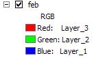
Select Feb layer in
Image analysis window and click on NDVI button ![]() under processing section. You will see
NDVI_feb layer is created in ArcMap. Green color shows presence of vegetation
and other colors show absence of green vegetation.
under processing section. You will see
NDVI_feb layer is created in ArcMap. Green color shows presence of vegetation
and other colors show absence of green vegetation.
Right click on the
NDVI_feb layer and data/export data. Chosse location to EX6 geodatabase and
Name as NDVI_feb. Repeat the same process to get the July NDVI and save the
data.
Q. What is the prominent difference between July and Feb NDVI for
Lancaster County? Zoon in near the airport area and compare your results with
false color composite image of same area that you have explored earlier? Do you
think NDVI values are affected by the clouds?
Part
III Image classification
Often we use readily
available data in GIS. This data is GIS ready and is provided by various
government agencies or private organization. Let’s see how this data is
obtained from imagery. We are going to create our own land use map as an
example. You have provided with Landsat 5 imagery for path 28 and row 32. This
covers area of Lancaster County, Nebraska where Lincoln is located. We will
start working with raw Landsat imagery and build our own land use map.
Landsat 5 has 7
bands as explained
at the beginning of the exercise. Each band contains reflectance within certain
wavelength. After we stack these bands we will have information from all the
bands contained within single image for entire area. These multiband images can
be used for creating spectral profile of the location in remote sensing
analysis.
Search for composite bands tool under tools option. Tool is located under data management\raster\raster processing\composite
bands. Select input rasters from
LT50280322005196EDC00 folder under
you exercise folder. This folder contains TIFF images for 7 landsat bands. Add
all 7 bands as input rasters. (Trick is to select first image
L5028032_03220050715_B10, hold shift key and select one.) Make sure all bands
are added in the same order (from L5028032_03220050715_B10 to
L5028032_03220050715_B70). Save the
output file as LandJulyComp.img under
Ex6 geodatabase. (Note: if it gives the error, you can save it under the
separate folder anywhere you want.)
This was the
conventional way of doing composite
bands. With Image analysis window you can do it on the fly. Add all the
seven landsat bands (from L5028032_03220050715_B10 to L5028032_03220050715_B70)
to ArcMap. With this tool you can create a composite band of any layers that
you want and perform image classification analysis on that.
Now reproject the LandJulyComp.img to NAD 1983 StatePlane Nebraska FIPS 2600
Feet. Search Project Raster. Select
input raster as LandJulyComp.img.
Name output raster dataset as ‘LandJulyCompProj.img’
under you exercise folder. Import coordinate system from the layer ‘NASS_2005’. Choose geographic
transformation as WGS_1984_ITRF00_To_NAD_1983.
Set RGB combination of LandJulyCompProj.img
as Layer4, Layer3, Layer2. This is
false color composite which
facilitates the green vegetation
identification. Red color shows the presence of green vegetation and green
color shows the absence of vegetation. Also observe the clouds with the white
color which are scattered over the image.
Clouds are masked
in remote sensing analysis to avoid error. Right
click on Ex6 geodatabase in ArCatalog.
Click new/feature class. Name is as Clouds
with alias Cloud. Choose type of feature as polygon. On next window import coordinate system from CALMIT_2005
raster in Lancaster geodatabase i.e NAD
1983 StatePlane Nebraska FIPS 2600 Feet. Now your empty polygon feature
class is ready and we will digitize the clouds. Add ‘clouds’ polygons to ArcMap.
On the editor
toolbar click Editor/start editing. Choose clouds
polygon. You will see white color
clouds scattered all over the image. Zoom in any of the cloud and observe you
will also see black color shadow of the cloud just on the northwest side of the
cloud. This is indication of the direction in which Landsat sensor has acquired
the image.
In the create
feature window choose cloud layer and in construction tools choose polygon. Now
approximately digitize the cloud and cloud shadow or five to six sizable clouds
in same area. Go to editor\ Stop editing
and save your edits. Once we have identified the clouds we need to
mask it (i.e. fill it with null/-9999 or similar value). In typical remote
sensing software (ERDAS Imagine or ENVI) cloud filling is one step operation.
In ArcGIS there is no direct way to
mask the clouds. However one can use model in model builder with various tools to mask the clouds. One such idea
is - Add new field to cloud polygon attribute table with -9999, Convert polygon
to raster using -9999 field, Use
conditional statement to get new raster which is cloud masked raster with cloud
value -9999, Use set null tool to set remove cloud part. Interested students
can follow similar approach, but it is not mandatory for this exercise. ArcGIS
has very powerful geoprocessing tools, students are encouraged to explore tools
for such analyses purposes.
Q.
Turn in the false color composite image with cloud polygon overlain on that. (use
thick contract boundaries for polygon with hollow symbology)
Next part is to
classify the image to create land use map. Go to Customize/Toolbars/Image Classification. Make sure Spatial Analyst extension is
enabled.

Turn all the layers off and make only three layers
visible - CALMIT_2005, NASS_200,
and LandCompJulyBandProj.img. Set
RGB combination of LandJulyCompProj.img as Layer4, Layer3, Layer2. This is false color composite which facilitates
the green vegetation identification. Red color shows the presence of green vegetation and green color shows the absence of vegetation.
Observed how urban
area in the middle of the image is green and agricultural fields outskirts are
red color. The landsat image is obtained in July, which is peak growing season
for corn and soybean – major crops
in the state. This will give you a feel how land use map of NASS and CALMIT in agreement with actual landsat image. You can also zoom in
use swipe layer tool in image
analysis window to see the detail of three images.
We are going to
perform image classification to make our own land use map and compare it with
CALMIT and NASS products.
Image
classification
refers to the task of extracting information classes from a multiband raster
image. Depending on the interaction between the analyst and the computer during
classification, there are two types of classification: supervised and unsupervised.
The intent of the classification process is to categorize all pixels in a
digital image into one of several classes,
or "themes". This
categorized data may then be used to produce thematic maps. (e.g. land cover) Normally, multispectral data are used to
perform the classification and, indeed, the spectral pattern present within the
data for each pixel is used as the numerical basis for categorization
(Lillesand and Kiefer, 1994).
Unsupervised
classification is a method which examines a large number of unknown pixels and divides
into a number of classed based on natural groupings present in the image
values. Unlike supervised classification, unsupervised classification does not
require analyst-specified training data. The basic premise is that values
within a given cover type should be close together in the measurement space
(i.e. have similar gray levels), whereas data in different classes should be
comparatively well separated (i.e. have very different gray levels) (PCI, 1997;
Lillesand and Kiefer, 1994; Eastman, 1995 )
The classes that result from unsupervised
classification are spectral classed which based on natural groupings of the
image values, the identity of the spectral class will not be initially known,
must compare classified data to some form of reference data (such as larger
scale imagery, maps, or site visits) to determine the identity and
informational values of the spectral classes. Thus, in the supervised approach,
to define useful information categories and then examine their spectral
separability; in the unsupervised approach the computer determines spectrally
separable class, and then define their information value. (PCI, 1997; Lillesand
and Kiefer, 1994)
Unsupervised classification is becoming
increasingly popular in agencies involved in long term GIS database
maintenance. The reason is that there are now systems that use clustering
procedures that are extremely fast and require little in the nature of
operational parameters. Thus it is becoming possible to train GIS analysis with
only a general familiarity with remote sensing to undertake classifications
that meet typical map accuracy standards. With suitable ground truth accuracy
assessment procedures, this tool can provide a remarkably rapid means of
producing quality land cover data on a continuing basis.
On the Image
Classification toolbar under classification choose Iso Cluster Unsupervised Classification. Make sure you have LandCompJulyProj.img layer selected for classification.
![]() . Select number of
classes as 20. Name out put
classified raster as ISO_Unsupervised.
Save output signature file as ISO_Unsupervised.gsg. Keep rest of the
options to default.
. Select number of
classes as 20. Name out put
classified raster as ISO_Unsupervised.
Save output signature file as ISO_Unsupervised.gsg. Keep rest of the
options to default.

This is first rough estimate of how your land use map might look like. We can use
this map now to see which pixels are grouped in one class and it will serve as
guideline for us to choose the training samples for supervised classification.
Training samples in supervised classification are input by user which serve as
a ground truth.
Let’s compare the land use map with CALMIT and NASS land use maps for 2005.
Use ![]() and
and ![]() buttons on Image Analysis window to compare
the three land use map. Zoon in various areas of the map to investigate in
detail. You can simply check and uncheck the layers in frame and compare the
display by toggling.
buttons on Image Analysis window to compare
the three land use map. Zoon in various areas of the map to investigate in
detail. You can simply check and uncheck the layers in frame and compare the
display by toggling.
Q. Turn in the output
of Iso Cluster Unsupervised Classification with class symbology shown on the
side. Comment on the comparison between three land use maps. Give the class
numbers (from ISO_Unsupervised layer) of the land use categories (from NASS or
CALMIT) that you think are quite well mapped by the unsupervised
classification. Which classes do you think are captured most accurately? Do you
think clouds will have impact on the classification? If yes, how? Do you think
clouds and cloud shadows are capture by the unsupervised classification? If
yes, give the class numbers.
Lets try supervised classification. We need
to create training dataset where we
will mark the areas on the image with known classes. In practice this data is
collected using GPS on the ground
and actual land use class is assigned to the point. Since we don’t have ground
truth data, we can use NASS and CALMIT landuse maps as a ground truth.
On the image classification toolbar make sure
LandCompJulyBandProj.img is active![]() . Now
click on ‘draw training sample with
polygon’ tool
. Now
click on ‘draw training sample with
polygon’ tool![]() .
.
Now we will draw polygons around some samples
of each land use class in CALMIT_2005 map. Let’s start with water. Zoom
in near branched oak lake area in
the image. If you see CALMIT_2005 map it is a large waterbody in northwest side of the image (most probably
shown in blue color).
Figure below shows the illustration of how to
draw the polygon. First image shows zoomed area of branched on lake from CALMIT_2005
layer. We are using this map as guideline to draw training sample, however we need to be careful of clouds.
Second image shows LandCompJulyBandProj.img in which cloud/cloud shadow is clearly shown on the lake. We will avoid
cloudy area while drawing polygon. Third image shows the sample training
polygon only drawn on cloud free lake area. We also need to draw a polygon well
within the CALMIT_2005 layer’s lake to avoid spectral mixing or mapping error
on the edges of CALMIT land use classes.
Now last image shows results of our ISO unsupervised classification, notice
how lake area is covered in bluish grey color and cloud is also captured in black color. You can see lake is
incorrectly mapped in unsupervised classification. This is an example of why
cloud masking is essential to avoid errors.
Now continue looking for water bodies in
CALMIT map and draw polygons within them avoiding clouds. You can toggle
between layers by turning layer on
and off. Trick is to keep only
required layers on and toggling between them. You can also use ![]() and
and ![]() buttons on Image Analysis window. After you
have drawn few polygons for water class, open training sample manager
buttons on Image Analysis window. After you
have drawn few polygons for water class, open training sample manager ![]() on image
classification window.
on image
classification window.
As shown below, I have drawn seven polygons
for water class. Select all your polygons for water class in training manager
using shift key and left mouse button. Click on the merge ![]() button. You just have merged all the polygons
into single polygon which all represents water body as your training data (ground truth). Click on the class name
‘class 1’ and rename it as Water, choose sky blue color under color column. You
have finished creating training sample for water with appropriate symbology.
button. You just have merged all the polygons
into single polygon which all represents water body as your training data (ground truth). Click on the class name
‘class 1’ and rename it as Water, choose sky blue color under color column. You
have finished creating training sample for water with appropriate symbology.
If you have incorrectly drawn the polygon, open training sample manager and
click on the record, it will highlight the selected polygon, simply
delete the polygon using ‘delete’
key or use ![]() button.
Note you have to do this before merging the polygons. You can also split your
merged samples using
button.
Note you have to do this before merging the polygons. You can also split your
merged samples using ![]() button and reinvestigate each polygon.
button and reinvestigate each polygon.
Above figures indicates the training samples for Irrigated corn, after I merged them I
created Irrigated Corn class. Click on the class in training manager and click on histogram
tool![]() .
Histograms for that class will be plotted (for each band in the layer) as shown
in figure above. Notice difference between histograms of each layer. Histogram
for layer 4 is normally distributed and have more pixels with high values. This
is near infrared (NIR) band in
Landsat which we use for vegetation
assessment (NDVI).
.
Histograms for that class will be plotted (for each band in the layer) as shown
in figure above. Notice difference between histograms of each layer. Histogram
for layer 4 is normally distributed and have more pixels with high values. This
is near infrared (NIR) band in
Landsat which we use for vegetation
assessment (NDVI).
Repeat the same process for few other classes
as shown the in the table below in CALMIT_2005
layer. Urban vegetation is a new
class you need to create which is not in CALMIT layer. CALMIT assigned urban
class to entire Lincoln area. However there are some trees and grass within the
city. Try to find it and assign it as Urban
Vegetation class.
|
Water |
Dryland Alfalfa |
|
Irrigated Corn |
Riperian Forest and
Woodland |
|
Dryland Corn |
Range, Pasture, Grass |
|
Irrigated Soybean |
Urban |
|
Dryland Soybean |
Urban Vegetation |
|
Irrigated Alfalfa |
Choose as many samples as you can for each
class and merge them, rename them, specify appropriate symbology.
Remember it is not important to just have
higher number of samples for good classification, but also to have reliable samples. So make sure you don’t have the cloudy area in you sample,
make sure you see the false color
composite (LandCompJulyBandProj.img) and choose nice consistent area for
samples using CALMIT land use map as a guideline. Also modify the symbology of
CAMLIT land use map to enhance current land use class that you are sampling (may
use dark/fluorescent colors). Use your intuition and knowledge of ArcGIS to get
best out of your image. Remember geography is both art and science.
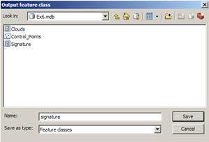
Once you have finished you samples for all 11 classes, use reset class values
button ![]() to arrange the class values. Notice class
values are now arranged in contiguous order. Use
to arrange the class values. Notice class
values are now arranged in contiguous order. Use ![]() button training
sample manager window to and save the output
feature class as ‘signature’ in
you Ex6 Geodatabase. Make sure Save as type is feature class and not shapefile.
Otherwise you won’t be able to save it Ex6 geodatabase.
button training
sample manager window to and save the output
feature class as ‘signature’ in
you Ex6 Geodatabase. Make sure Save as type is feature class and not shapefile.
Otherwise you won’t be able to save it Ex6 geodatabase.
Also save the signature file using ![]() button on training
sample manager window, name it as ‘SupervizedSiganture’.
This file will have .gsg extension. Note that you can’t really save signature
file in Ex6 geodatabase. So you can save it anywhere in your folder.
button on training
sample manager window, name it as ‘SupervizedSiganture’.
This file will have .gsg extension. Note that you can’t really save signature
file in Ex6 geodatabase. So you can save it anywhere in your folder.
Select all the 11 classes and click on scatterplots ![]() button.
Scatterplot of various layers will be displayed.
button.
Scatterplot of various layers will be displayed.
Close the training sample manager.
On Image Classification window, under classification choose interactive supervised classification.
Map layer will be created using training samples that you just created. New
layer named Classification_LandCompJulyBandProj.img
will be created, which is your land use map.
Note: Do not panic if you see your land use map looks very weird or
shows only single value/class for entire map. It is likely if you choose very
fewer samples or samples which are wrong or which are under cloud cover. You
can again open training sample manager and revise your samples. Focus on the
classes which you have created with very few samples (Check the count column in training sample
manager)

You just have created your own Landuse map. Although ArcMap shows the legend, it is not present in
the attribute table of the layer. Open attribute table of the layer ‘Classification_LandCompJulyBandProj.img’
Notice Class_Name
is described as Class_1, Class_2 etc.
Let’s save this layer first. Right click on the ‘Classification_LandCompJulyBandProj.img’ layer select Data/Export data. Select Name as
Classification_LandCompJulyBandProj
and Location to Ex6 geodatabase. Leave rest of the options to default. After saving
add the layer to ArcMap. Remove old temporary file Classification_LandCompJulyBandProj.img’from ArcMap.
We need to make it as actual classes. Open ‘Signature’
feature class from Ex6 geodatabase.
Right click on Classification_LandCompJulyBandProj’
layer, click Joins and Relates/Join.
Join attribute from a table with ‘value’
and choose table to join this layer as ‘signature’,
choose field in the table to base the join on as ‘Classvalue’. Keep all the records.
Open the attribute
table of Classification_LandCompJulyBandProj
after joining and make sure it is joined correctly. You should now see actual classnames like water, irrigated corn etc.
Right click on the Classification_LandCompJulyBandProj layer and Data/Export Data. Save it under Ex6 folder under the name ‘Classification_LandCompJulyBandProjJoin’.
Add Classification_LandCompJulyBandProjJoin’
to the ArcMap. Change the symbololy
of the layer. Chose unique values
with value field ‘classname’
Q. Turn in the
supervised classification map with class names shown in the legend. Visually
compare the map with CALMIT 2005 and NASS maps and comment on how accurately
you have classified the maps.
Now we will perform maximum likelihood classification. On Image Classification window
select Classification/ Maximum
Likelihood Classification. Select input raster band as ‘LandCompJulyBandProj.img’ Choose
signature file ‘supervizedsiganture.gsg’
that you have saved earlier. Save the data under Ex6 geodatabase with the name ‘MLC_Lancaster’. Leave rest of the options
as default.
Q. Turn in the maximum likelihood
classification map with class values
shown in the legend. Visually compare the map with CALMIT 2005 and NASS maps
and comment on similarity or differences in the map classes.Could you relate to
some class values (from MLC_Lancaster) to classnames (in Landuse_2005)
Now we will compute the class probability. On Image Classification window select Classification/ Class Probability.
Select input raster band as ‘LandCompJulyBandProj.img’
Choose signature file ‘supervizedsiganture.gsg’ that you have saved earlier. Save
the data under Ex6 geodatabase with
the name ‘CP_Lancaster’. Leave rest
of the options as default.
Output will contain 11 bands. There is one band for each class or cluster in the input
signature file. Each band stores the probability that a cell belongs to
that class. This can be useful in merging classes after a classification is
done.
Learn
more about Class probability by searching in ArcGIS help ![]() .
.
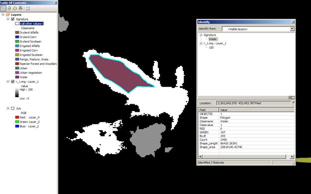
After you run class probability tool, ‘CP_Lancaster’ layer will be added to
the map. This is three band layer. But actually there are 11 bands created, one
for each class of signature file. Navigate to ‘CP_Lancaster’ layer in Ex6 geodatabase and double click on the file
(do not add to map). Now you will see the 11
layers with names Layer_1, Layer_2
and so on. Open each of the layers in ArcMap and observed how it probability is high where the
class features are present. Open the ‘signature
feature class’ from Ex6 geodatabase.
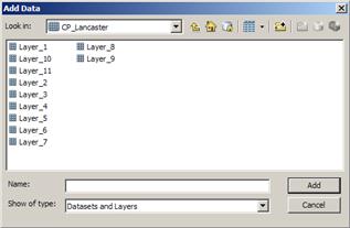
Open attribute table of the layer ‘signature’ Select the attribute ‘water’ and open the layer that
corresponds to it (if it is first class in attribute table it will be ‘layer_1’). Observe how probability
is 100% where your signature file
has ‘water’ class polygon.
Q. Turn in the screenshot zoomed in one of
your polygon for ‘urban vegetation’ class from signature file with map of class
probability for urban vegetation class.
Q. Also turn in the
full extent map of ‘urban vegetation’ class probability and compare it with the
CALMIT land use map. Comment how your ‘urban vegetation’ class is mapped
compared to Landuse map of CALMIT (note CALMIT does not have this class, so see
what corresponds in CALMIT map for your ‘urban vegetation’. What do you think
are the possible errors in the mapping ‘urban vegetation’? What could be the
reasons?
Open the attribte tables of the three layers ISO_Unsupervised, CALMIT_2005,
Classification_LandCompJulyBandProjJoin and MLC_Lancaster. Export the attribute tables with
corresponding names in your folder. Open it using MS Excel. Create the histogram
each land use class/value using
count.
Here count is a pixel count in that class.
Each pixel is ~98 feet. So are of land use can be computed as pixel count
multiplied by 98 * 98. (This is informational you need not compute the area)
Q. Turn in histogram
of each land use map. Compare and comment on the histograms. This is sort of
comparison for each land use classification we have performed.
References
http://www.sc.chula.ac.th/courseware/2309507/Lecture/remote18.htm
http://www.youtube.com/watch?v=xVVdZOQiBuQ&feature=related
ArcGIS 10 help
ESRI training Visualizing and Analyzing Imagery with ArcGIS 10
Esri Training | Georeferencing Rasters in
ArcGIS