Computing Water Surface Elevation with HEC-RAS
Prepared by David R. Maidment and Gonzalo Espinoza
CE 374K Hydrology
Spring 2011
Starting a
HEC-RAS Project
Channel
Geometry
Flow Data
Steady Flow
Simulation
Summary of
Items to be Turned In
The goal of this exercise is to give you and understanding of how the HEC-RAS model is run for steady flow profiles on Waller Creek. The model’s geometry data and steady flow data is provided for you in the http://www.caee.utexas.edu/prof/maidment/CE374KSpring2011/HECRAS/wallerras.zip file. Obtain these files and put them in a working directory on your computer. You should see the following file list:
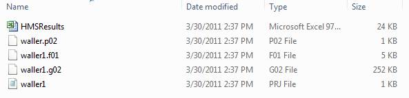
HMSResults.xls is a file of
discharges at various points along Waller Creek and its tributary (the Hemphill
Branch) computed from the HEC-HMS model that you worked with in the previous
homework exercise. We won’t use this
file except as a reference so you can see the link between the HEC-HMS and
HEC-RAS models.
Waller1.f01 is a Flow File used as input to HEC-RAS,
developed from the flows in the HMSResults.xls spreadsheet
Waller1.g02 is a Geometry File describing the river
channel and bridges on Waller Creek
Waller1.prj is a Project File that controls how HEC-RAS
runs
Waller1.p02 is a set of parameters
for the water surface profile computation
The HEC-RAS Version 4.1 program is accessible in ECJ 3.302 and can also be obtained directly from HEC at http://www.hec.usace.army.mil/software/hec-ras/
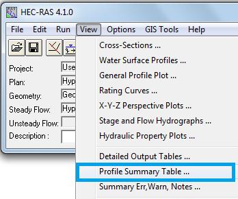
To open HEC-RAS, look for a folder called “HEC” from the Start button on your computer, there should be a HEC-RAS 4.1.0 icon.
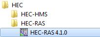
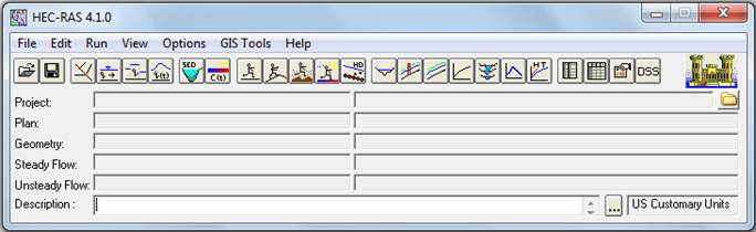
Double click the icon to open the main project window, which looks like this:
Click on the Open Project… command from the File menu. Scroll down to your working directory and highlight the project titled “Use of GeoRAS Input”, file waller1.prj. Click OK. The Project, Geometry, and Steady Flow information lines should now be filled with the titles of those respective files as shown:
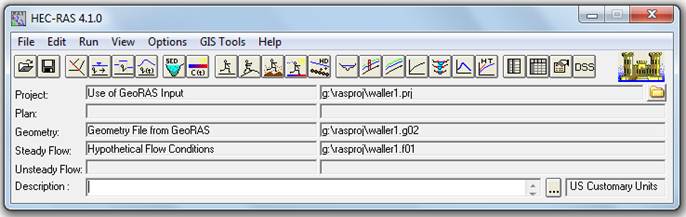
As shown in the main menu, four files are required to run a HEC-RAS project. First, the Project File acts as a file management tool and identifies which files are used in the model. The Plan File sets the model conditions as subcritical, supercritical, or mixed flow and runs the simulation. The Geometry File contains all the geometric attributes for the model (which, for our case, are imported from GIS using GeoRAS). Lastly, the Steady Flow File establishes the steady-state flow and boundary conditions at numerous points in time for the model. Disregard the Unsteady Flow information line for the moment.
Let’s first examine the geometry data that was developed using the same methodology we used in the previous section. Select Edit/Geometric Data… from the main project window.

What you see is the plan view of a set of cross-sections on Waller Creek,
with labels measuring the River Station,
or distance in feet from the downstream end of the creek. River Stationing on the Waller Creek starts at the
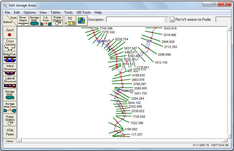
To be turned in: What is the total routing distance in feet
simulated by this model (i) for Waller Creek, (ii) for the tributary?
Details of the Geometry Data can be examined from this window. Click on the Cross Section button to
see the tabular data for each cross section.
![]()
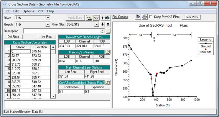
In this case, we are looking at the Cross-section at River Station 3543.919 on the Trib reach. The points defining the cross-section are shown in the table to the left and plotted in the graph to the right. In the table, Station refers to the distance from the left side of the cross-section (looking downstream), measured in feet, while Elevation is the elevation above mean sea level in feet. The Downstream Reach Lengths refer to the distance in feet to the next downstream cross-section, the Manning’s n Values are the n values for the Left Overbank (LOB), Channel, and Right Overbank (ROB), respectively. The Main Channel Bank Stations refer to the Station values of the two red dots in the plot, and the Contraction and Expansion Coefficients refer to the coefficients for the minor head losses associated with changes in channel cross-section.
Control structures along a stream can be manually entered using the
corresponding buttons from this editor.
We will not be using any control structures for this model. You can move around on the routing reach
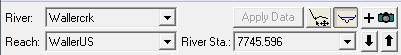
using the ![]() arrow keys, and you can change what river and
what reach of the river you are on with the tab buttons,
arrow keys, and you can change what river and
what reach of the river you are on with the tab buttons, ![]() ,
as shown below. You can use the
,
as shown below. You can use the ![]() button to toggle the plot display on or off.
button to toggle the plot display on or off.
To be turned in: How many routing reaches are there in this
model? What are their names?
In the Cross Section Data window, use the ![]() button to copy the cross section plot to the
clipboard. From there, you can paste it
into your homework solution.
button to copy the cross section plot to the
clipboard. From there, you can paste it
into your homework solution.

To be turned in: Take
Cross-section 7426.129 on the WallerUS reach of the
(a) Width
of the cross-section in feet
(b) Stationing
on the cross-section of the left bank and right bank of the channel, in feet,
and elevation of these points in feet above mean sea level.
(c) The
Manning’s “n” values used at this cross-section for left overbank, channel and
right overbank flow.
(d) The
distance in feet to the next downstream cross-section.
(e) The
river station in feet of the next downstream cross-section
Close the Cross Section Data and Geometry Data windows so that you get back to the main River Analysis System window. We are now ready to input the flow data for the model.
The flow data has been extracted from a HEC-HMS hydrologic model of the
First, let’s open the Steady Flow Editor. Select the Steady Flow Data… command
from the Edit menu.

The Steady Flow Editor should look like the following. The locations shown are the River Stations at which the discharge is changed.
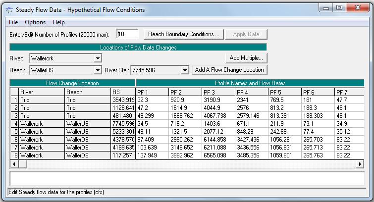
There are three sections of Steady Flow Data that have been inputted using this window: Enter/Edit Number of Profiles, Flow Change Location/Profile Names and Flow Rates, and Reach Boundary Conditions.
Enter/Edit Number of Profiles
A “Profile” is a list of flow conditions at specified locations along the extent of the model’s reaches at a specified point in time. Each entered Flow Profile will result in a steady-state water surface profile along the length of each reach. Open completion of running the model (which we will do in the next section) results can be observed from the View Profiles, View Cross Sections, or View 3D Multiple Cross Section Plot buttons provided in the HEC-RAS Main Menu window.
For this exercise, a total of ten profiles were entered. The profiles correspond with flow data extracted from the HMSResults.xls file at one-hour time intervals, at 0100 hours, 0200 hours, 0300 hours, and so on.
Open Flow Data
The editor initially showed the upstream cross sections of each reach in the model: cross sections 3543.919 (upstream boundary of the Tributary), 7745.596 (upstream boundary of WallerUS), and 4378.570 (upstream boundary of WallerDS). In addition, the cross sections acting as outlets of watersheds for rainfall runoff were added as well. If you examine the spreadsheet, HMSResults.xls, you will find flow data for upstream boundaries as well as runoff data for specified cross sections along both Waller Creek and the Tributary. This data was used for this model. When adding the flow data to HEC-RAS, the values entered for a specified cross section is an accumulated flow. All flows upstream of a flow change location in the model must be added to the flow at that point. In other words, the model is obtaining a “snapshot” in time of the flow at locations along each reach to develop the water surface profiles.
Reach Boundary Conditions
The final step in the Steady Flow Data development is establishing the Reach Boundary Conditions. Click on the Reach Boundary Conditions button. The Steady Flow Boundary Conditions Editor is used to set the water surface elevation boundary conditions. Click in the “Known WS” cell in the Downstream column. Notice that the water surface elevation for cross section 14.035 on “WallerDS” is inputted for each profile, establishing the boundary conditions for each steady-state profile. The Junction = 2 in this table specifies that the Trib, WallerUS and WallerDS, join at a single junction, so that the downstream boundary condition for the Trib and WallerUS is established by the water surface elevation at the upper end of the WallerDS reach.

To be turned in: What is the water surface elevation of the
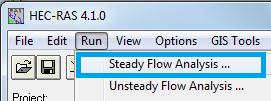
We are now ready to run a Steady-State Flow simulation. From the Run menu, select Steady Flow Analysis.
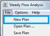
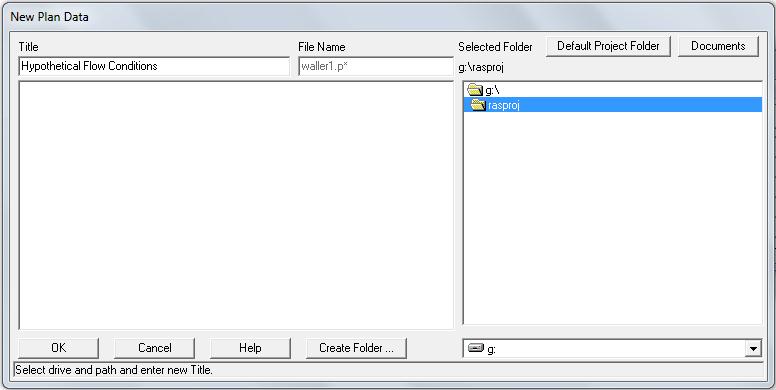
Under the File menu, select New Plan. Enter “Hypothetical flow conditions” as the Plan’s title and put into the next window which appears a 12-character short identifier, “Hypoflow”. Click OK.

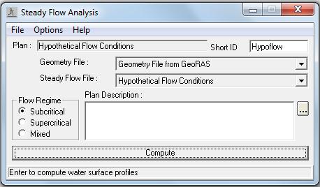
Ensure the Flow Regime is set to Subcritical and press the COMPUTE button. This starts a FORTRAN program called SNET, which carries out all the calculations for the simulation.
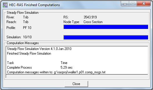
Close the Finished Computations window, and the Steady Flow Analysis window.
You can see the results of the model using the View/Water Surface Profiles button.
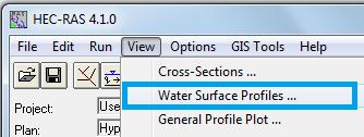
From the Profiles menu you can select a particular water surface profile, and from the Reaches menu, you can see the profile in each of the computational reaches.
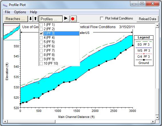
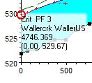
If you click on a point on this profile, you can read the stationing the flow and the water surface elevation:
To be turned in: Locate the three cross-sections closest to
the junction of the
You can use the “Animate the simulation results” ![]() button to show the time sequence of the water
surface profiles in any reach.
button to show the time sequence of the water
surface profiles in any reach.
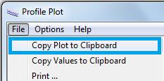
You can use File/Copy Plot to Clipboard to save a copy of the Profile Plot and paste it into your homework solution.
In the View / Water Surface Profiles
menu, select Profile 3, and the Waller US reach, then select View/Profile Summary Table
The resulting table for WallerDS shows summary data about the water surface
profile.

To be turned in: For Profile 3 and Cross-section
7426.129 on the WallerUS reach of the Wallercrk River, make a plot of the water surface profile
using HEC-RAS, and use the Summary Table to find the following:
(a) Discharge
(cfs), Minimum channel elevation, water surface
elevation, elevation and slope of the energy grade line, and the velocity in
the channel.
(b) Determine from these quantities, the values of the terms in the energy equation: H = z + y + V2/2g. Assume z is at the minimum channel elevation. What is the elevation of the Hydraulic Grade Line at this location? What flow condition prevails here? Is the assumption of Subcritical flow throughout the profile correct?
Ok, you’re done! Save the Project and close all the Windows.
Summary of items to be
turned in:
(1) What is the total routing distance in feet
simulated by this model (i) for Waller Creek, (ii) for the tributary?
(2)
How many routing reaches are there in this model? What are their names?
(3)
Take Cross-section 7426.129 on
the WallerUS reach of the
(a) Width
of the cross-section in feet
(b) Stationing
on the cross-section of the left bank and right bank of the channel, in feet,
and elevation of these points in feet above mean sea level.
(c) The
Manning’s “n” values used at this cross-section for left overbank, channel and
right overbank flow.
(d) The
distance in feet to the next downstream cross-section.
(e) The
river station in feet of the next downstream cross-section
(4)
What is the water surface elevation in feet above mean sea level of the
(5)
Locate the three cross-sections closest to the junction of the
(6)
For Profile 3 and Cross-section 7426.129 on the WallerUS reach of the
(c) Discharge
(cfs), Minimum channel elevation, water surface
elevation, elevation and slope of the energy grade line, and the velocity in
the channel.
(d) Determine from these quantities, the values of the terms in the energy equation: H = z + y + V2/2g. Assume z is at the minimum channel elevation. What is the elevation of the Hydraulic Grade Line at this location? What flow condition prevails here? Is the assumption of Subcritical flow throughout the profile correct?
Return to Dr Maidment’s Home Page