Building an Arc Hydro
Framework
with Time Series Geodatabase
Prepared by David R. Maidment and Jonathan L.
Goodall
GIS in Water Resources
Fall 2005
Goal
The goal of this exercise is to build a geodatabase for the
Overview of what is to be done
1.� How to
create HydroJunctions for the USGS streamflow gaging stations using linear
referencing and the National Hydrography Dataset flow lines.
2.� How to populate
an Arc Hydro geodatabase with spatial and temporal information for a particular
river basin.
3.� Show
examples of vector-based analysis available in ArcGIS software for hydrologic
data.� Specifically, we will introduce
the Utility Network Analyst and TrackingAnalyst extensions.
Computer
and Data Requirements
To carry out this exercise, you need to have a
computer, which runs the ArcInfo
version of ArcGIS. The data are provided in the accompanying zip file, http://www.ce.utexas.edu/prof/maidment/giswr2005/ex4/ex4.zip��
Data description:
Ex4.zip contains a geodatabse with feature classes
that we will use in this exercise.� To
start this exercise extract the entire contents of the zip file to a convenient
location (e.g. C:\temp\Ex4)
The contents of the zip file are shown:
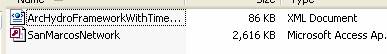
and the geodatabase SanMarcosNetwork looks like:
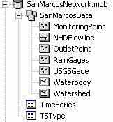
The SanMarcosNetwork personal geodatabase contains the
following
�
A
feature dataset "SanMarcosData" that contains the feature classes NHDFlowline, USGSGage, RainGages, OutletPoint, MonitoringPoint, Watershed,
and Waterbody.
�
A
table "TimeSeries"
comprising daily rainfall data from the National Climate Data Center (NCDC) and
daily streamflow data from the USGS.
�
A
table TSType with metadata for the
daily rainfall and streamflow time series records.
The NHDFlowline and Waterbody feature classes are obtained from the Medium Resolution
(1:100,000 scale) National Hydrography Dataset for the San Marcos HUC
(12100203).� The instructions for
obtaining these data are given in NED_NHD.doc.� The High Resolution (1:24,000 scale) NHD data
are available for this HUC but they are not used in this exercise because
applying flow direction to them takes a long time and we wanted streamline this
exercise.��� The USGSGage feature class includes only those USGS gages that are
currently active in the
River Addressing
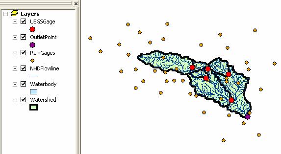
River addressing refers to the location of objects on a river line feature class using measure values defined on the line vertices.� Let�s examine how this works for the National Hydrography Dataset.�� Open ArcMap and add from the SanMarcosData feature dataset the themes Watershed, Waterbody, USGSGage, RainGages, OutletPoint and NHDFlowline.�� Pretty neat!
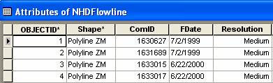
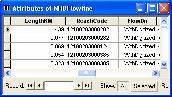
If you open the Attribute Table for NHDFLowline you�ll see that its Shape is PolylineZM, which means that its vertices can have (x,y,z,m) values where m is the Measure value along the line.
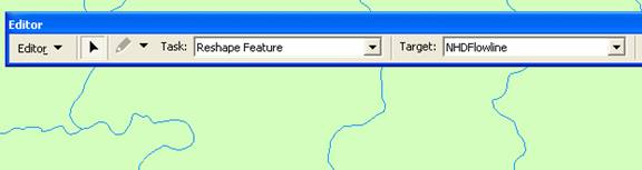
Open the Editor menu (use View/Toolbars/Editor to get toolbar), start editing, make SanMarcosNetwork the database to be edited, NHDFlowline the target feature class, Reshape Feature the edit task.��
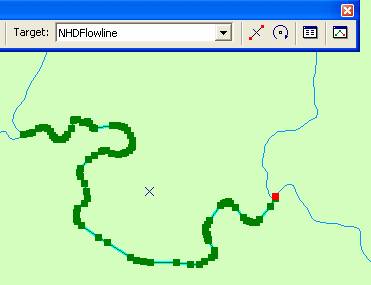
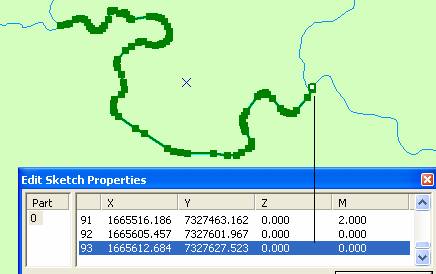
You�ll see a black triangular cursor.�� Zoom in on a stream line and double click on it (repeat the clicking a few times if at first it doesn�t work).�� You should see the vertices on the line highlighted.
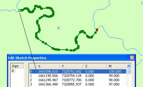
Click on the Sketch Properties tool ![]() �at the end of the Editor toolbar and open the Edit Sketch Properties palette.� If you click on the first row of the display,
you�ll see the first vertex of the line highlight.�� The X and Y values are the Easting and
Northing of this point in the coordinate system of the data.�� The M-value of this point is the percent
distance along the line, as measured from its downstream end.�� The value show is at 100%, which means that
it is at the most upstream end of the line.
�at the end of the Editor toolbar and open the Edit Sketch Properties palette.� If you click on the first row of the display,
you�ll see the first vertex of the line highlight.�� The X and Y values are the Easting and
Northing of this point in the coordinate system of the data.�� The M-value of this point is the percent
distance along the line, as measured from its downstream end.�� The value show is at 100%, which means that
it is at the most upstream end of the line.
If you scroll down through the table, you can identify intermediate points along the line
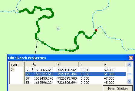
and the vertex at the most downstream end of the line
Close the Edit Session and Do Not Save your edits as we don�t want to disturb the dataset!

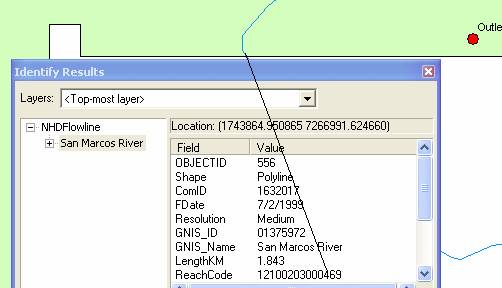
If you use the Identify tool ![]() �and click on the same stream line, you�ll get
its NHD attributes
�and click on the same stream line, you�ll get
its NHD attributes

The particular reach shown is on the
Linear Referencing on
Rivers
Now that we have a river addressing system, we can locate
features along the river.� Lets do that
for our USGSGages and watershed OutletPoint.��
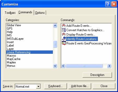
First lets locate a tool that identify measure values.��� Use Tools/Customize/Commands
and select the Linear Referencing
tools option and drag the Identify Route
Locations tool ![]() �onto your ArcMap toolbar display.�
�onto your ArcMap toolbar display.�
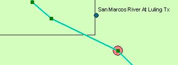
If you zoom to the location of the outlet of the basin, you can click on the NHD streamline there and you�ll see a measure value 18.785

A query similarly executed with the Identify Tool shows that this is Reach 12100203000469.�� Thus the river address (ReachCode, Measure) is (12100203000469, 18.785) for this location.�� Don�t worry if you don�t get precisely 18.785, you�ll get a value close to this.
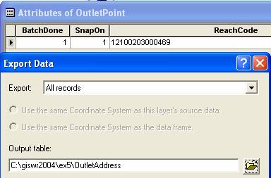
Lets store the river address of the OutletPoint in its attribute table.�� Open the Attribute Table for the OutletPoint and add a field ReachCode as type Text and Measure as type Float.��
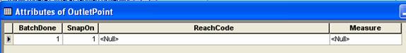
Start Editing this feature class, and type in the values for the river address:

Once the values are entered select Stop Editing and Save Edits.� We can now Display Route Events (the Reach is the Route and the Event is the point location on the route).� To do this, we need to show the events in a separate table.�� With the Attributes of OutletPoint table open, use Options/Export, to export the table as a separate dbase table called OutletAddress.� Say Yes, when you are asked whether to add this table to the map.�
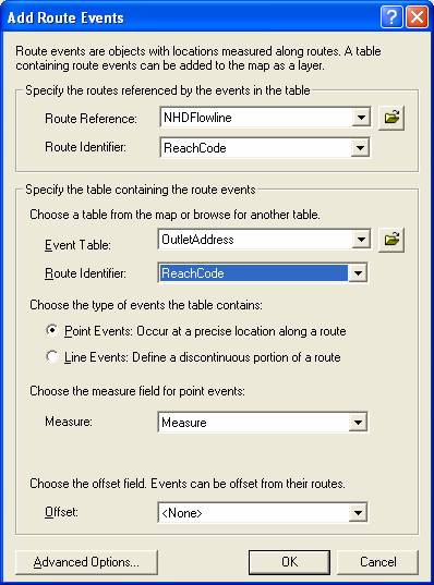
�Now, in ArcMap, use Tools/Add Route Events��
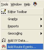
to display this event as a point on the map
Notice how the new outlet event falls precisely on the streamline.� This is very neat because it allows us to �locate� things along rivers without having to have the original reference point right on the river line itself.��
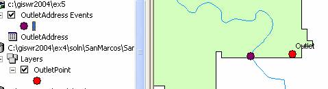
Right click on OutletAddress Events and use Export/Data to export the point to a new feature class called OutletAddressPoint in the SanMarcosData feature dataset.�
Ok, now its your turn to do some things.�� Please complete the river addressing for the 5 USGS Stream gages by the same method that you have just carried out for the outletpoint.� Store the result as the feature class StreamGageAddressPoint in the San Marcos Network feature dataset.� You may notice when you examine the ArcMap display that the route event doesn�t display quite where you thought it might, but actually on top of the nearest vertex to your route address.� Save your map document and close Arc Map.
To be turned in:� A screen capture of the attribute table of
the StreamGageAddressPoint feature class and a screen capture showing one of
the USGS gages with its corresponding stream address point located on the stream
line.
Building an Arc Hydro Geodatabase
Now that we have these address points processed, we are ready to build an Arc Hydro geodatabase.� In this exercise we will use the Arc Hydro Framework with Time Series schema.� The framework schema provides a simplified version of the full Arc Hydro schema.� There are a number of approaches for building an Arc Hydro geodatabase.� We will take the approach of first creating an empty geodatabase and then loading features into the certain feature classes within the geodatabase.��
We will use ArcCatalog to build the geodatabase, so close ArcMap and open ArcCatalog.
In your working directory, create a new personal geodatabase and name it SanMarcos_ArcHydro.mdb
Now we are going to apply the Arc Hydro schema to this
geodatabase.� The schema is stored in an
xml file provided with the exercise documents.�
You should be able to see the xml file from ArcCatalog (ArcHydroFrameworkWithTimeSeries.xml).� Double
click on the xml file to open the document in a web browser.�
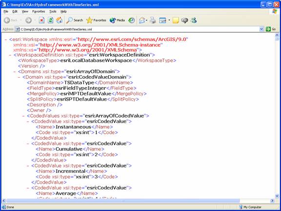
This xml file describes the feature classes, tables, fields, and relationships defined in the Arc Hydro with Time Series schema as depicted in Chapters 2 and 7 of the Arc Hydro book.�
To apply the schema to the empty geodatabase we just created, right-click on the geodatabase and select Import/XML Workspace Document.�
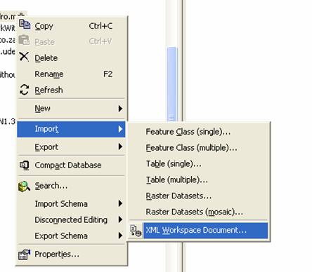
Choose to import only a schema and browse to the ArcHydroFrameworkWithTimeSeries.xml file.�
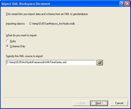
Press Next and then
Finish.
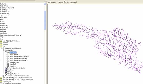
Refresh ArcCatalog (this step is very important or you won�t be able to see your result!) and then look at the SanMarcos_ArcHydro geodatabase.� Notice the structure of the geodatabase.� Preview one of the feature classes�s attribute table (while a feature class is selected, on the right side of ArcCatalog, select the Preview tab.� At the bottom of this tab, choose to preview the table instead of the geography.� You will notice that there are no features in the feature class, but that the feature class has Arc Hydro attributes� (HydroID, HydroCode, etc.).
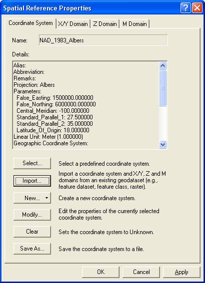
Before we import data, it is smart to first define the coordinate system of the ArcHydro feature dataset.� To do this, we will import the coordinate system of the SanMarcosData feature dataset in the SanMarcosNetwork geodatabase provided with the exercise.�
Right-click on the ArcHydro feature dataset and select Properties, then Edit the spatial reference.� Import the coordinate system of the SanMarcosData feature dataset in the SanMarcosNetwork geodatabase.� The coordinate system has the following attributes.�� Please note that there was a coordinate system (the USGS National Albers projection) contained in the XML document that you imported to the geodatabase.� We are replacing that with the coordinate system used for the rest of the data (the Texas Centric Mapping System).
 �
�
Ok, now let�s import some data.� One complication is that you are not able to import features into a feature class that is part of a geometric network.� That means we have to break the geometric network, import features into HydroEdge and HydroJunction, and then rebuild the network.
Delete the
HydroNetwork geometric network.� You
can do this by right-clicking and highlighting the HydroNetwork ![]() and pressing
the delete key.
and pressing
the delete key.
We are going to populate the feature classes within our geodatabase by loading data from another feature class.� This is a very useful procedure so it is good to get some practice at using it.
First we are going to load data from the NHDFlowline feature class in the SanMarcosNetwork geodatabase into the HydroEdge feature class in the SanMarcos_ArcHydro geodatabase.
Right-click on the HydroEdge feature class and select Load/Load Data.� (If you see the Load Data button greyed out, it is because you haven�t deleted the HydroNetwork.�� You can�t load data directly into a Network feature class, only to a simple feature class).
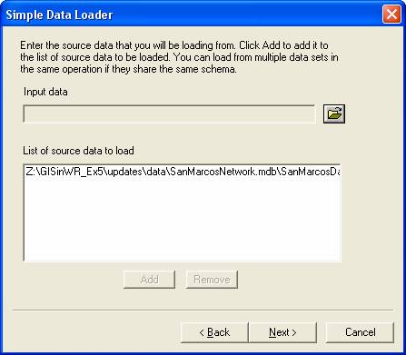
Browse to the NHDFlowline feature class within the SanMarcosNetwork geodatabase.� Press Add and then Next.�
Keep the defaults on the next window (you do not want to load the data into a subtype). Press Next.
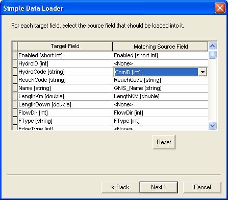
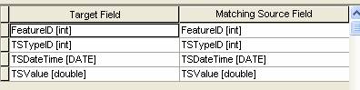
On the next window, make one change.� Set the matching source field for HydroCode to be ComID.� The ComID is a unique identified for NHD reaches, so it makes sense to use this as the HydroCode. Press Next.
Keep the default on the next window (Load all the source data).� Press Next.
Press Finish to complete the data load.
Once the process has completed, refresh your geodatabase.� You should see the HydroEdge class now populated.
Now let�s do the HydroJunction feature class.� We are going to load two feature classes into HydroJunction: StreamGageAddressPoint and OutletPointAddressPoint.�
First we�ll load
StreamGageAddressPoint.
Right-click on HydroJunction
in the SanMarcos_ArcHydro geodatabase and select Load/Load Data.� ��
Browse to StreamGageAddressPoint in the SanMarcosNetwork geodatabase.
Click Add and
then Next.
Match up the fields
as shown below:
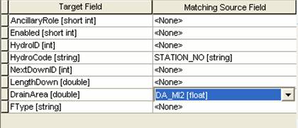
We are using Station_No as the HydroJunction�s HydroCode.� This will provide a link between Arc Hydro and data stored outside ArcHydro (like NWIS data) that is reference to a stream gage by its station number.
Click Next and then Finish to complete the data import.
If you mess up in any of these data loading steps, or inadvertently load the data twice, Open ArcMap, start the Editor and edit out the records or features that you don�t want.
So far so good.� Now let�s add the second feature class to HydroJunction: OutletAddressPoint.�
Right-click on HydroJunction in the SanMarcos_ArcHydro geodatabase and select Load/Load Data.�
Browse to OutletAddressPoint in the SanMarcosNetwork geodatabase.
Click Add and then Next.
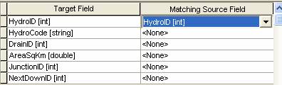
We do not want to transfer any of the fields from Outlet AddressPoint into HydroJunction.
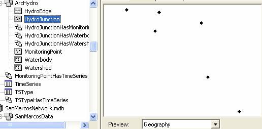
That�s it for HydroJunction.� You should have six features in the feature class now.� Five will be USGS stream flow gages and the sixth the basin outlet.� Its best to check this in the Geographic View since the sixth feature doesn�t seem to show up in the tabular view.
The MonitoringPoint features will come from the MonitoringPoint feature class (this feature class contains the USGSGage and RainGages feature classes and has the proper HydroIDs that link the MonitoringPoints to TimeSeries records).� Some preprocessing of the linkage between the spatial features and time series data has been done here to facilitate you doing this exercise readily.
Follow the same procedure as with the HydroEdge and HydroJunction.�
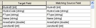
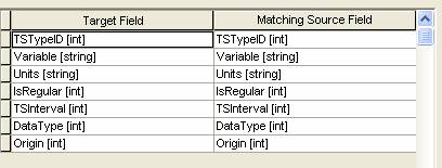
The fields for the MonitoringPoint feature class are:

We are also going to load the Watershed and Waterbody feature classes from the SanMarcosNetwork geodatabase into the Watershed and Watererbody feature classes in the SanMarcos_ArcHydro geodatabase.
The fields for the Watershed feature class are:
The fields for the Waterbody feature class are:
Finally, we need to
load in data from TimeSeries and TSType tables.�
The fields for the TimeSeries table are:
The fields for the TSType table are:
That�s it for ArcCatalog.� We have all of our data loaded into our geodatabase.� Next we need to populate some of the attributes in the feature classes.�
Populating Attributes
There are a few key relationships in ArcHydro that we will demonstrate in this exercise.� One is WatershedHasHydroJunction, MonitoringPointHasHydroJunction, and MonitoringPointHasTimeSeries.� To make these relationships functional, we must first populate a few fields within the Watershed, MonitoringPoint, and HydroJunction Feature Classes.
Close ArcCatalog
and open ArcMap.
Add all of the ArcHydro feature dataset and the TimeSeries and TSType tables to ArcMap.
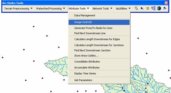
Add the Arc Hydro Toolbar if you haven�t already.
We are going to give HydroIDs to all of the feature classes, except for MonitoringPoint, HydroIDs.� (We aren�t going to give MonitoringPoint features HydroIDs because they already have HydroIDs and are related to TimeSeries records).
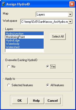
Under Attribute Tools on the Arc Hydro toolbar, select Assign HydroID.
Select all the layers
except for MonitoringPoint.� Choose
to overwrite existing HydroIDs and
to apply the procedure to all features.� Press OK.
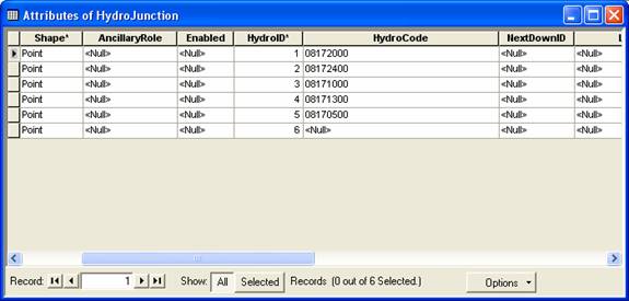
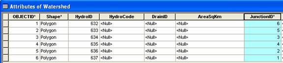
You can see that all of the features now have HydroID populated.� Here�s a look at the HydroJunction feature class:
Now we are going to use the Assign Related Identifier tool ![]() �to link the MonitoringPoint features with
their associated HydroJunction features.�
�to link the MonitoringPoint features with
their associated HydroJunction features.�
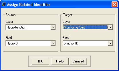
Select the ![]() �tool from the Arc Hydro toolbar.� In the pop-up window, choose the source to be HydroJunction�s HydroID and the
target to be MonitoringPoint�s
JunctionID.� Press OK.
�tool from the Arc Hydro toolbar.� In the pop-up window, choose the source to be HydroJunction�s HydroID and the
target to be MonitoringPoint�s
JunctionID.� Press OK.
This tool will populate a MonitoringPoint feature�s JunctionID attribute with a HydroJunction�s HydroID, thus establishing a relationship between the two features.
Now, zoom in to one
of the monitoring points, and then select the ![]() �tool again.�
You�ll see the same pop-up menu, but the tool remembers the Target layer
and field we just set so you can press OK.
�tool again.�
You�ll see the same pop-up menu, but the tool remembers the Target layer
and field we just set so you can press OK.
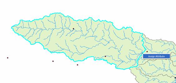
This tool is a little trick to get a handle, so be patient.� First select the MonitoringPoint feature.� Once this is selected, then right-click on the HydroJunction feature.� You should see an Assign Attribute box pop-up.� Click on the Assign Attribute box.� Once you do so, you�ll see both features flash indicating that the MonitoringPoint feature�s JunctionID has been set.�

Do this same procedure for the four other MonitoringPoint features.�
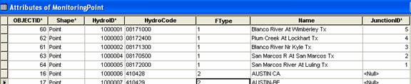
If you check the attribute table for Monitoring Points, you�ll see that the JunctionID has been assigned for those MonitoringPoints that are streamgages.
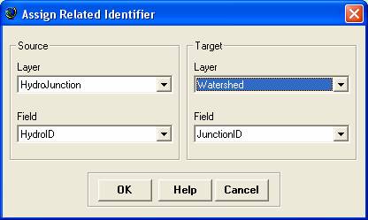
Ok, next we are going to use the same Assign Related Identifier tool to link the Watershed features with their HydroJunction outlet points.� Press the Assign Related Identifier tool and select the target layer to be Watershed and the target field to be JunctionID.� Keep the Source layer and fields as the layer HydroJunction and field HydroID that we set before.
Now, click on a watershed feature, then right-click on its outlet HydroJunction and press Assign Attribute.� Check to make sure the Watershed�s JunctionID is the HydroJunction�s HydroID.�
Follow this same procedure for each of the watersheds, being sure to also include the outlet and most downstream watershed.
Here�s what the attribute table should now look like for the watersheds.
That�s it for data manipulation.� We are now ready to do some analysis.
River Networks
Now we�re going to have some fun with the stream lines as a river network.�� Close ArcMap, Open Arc Catalog and examine the SanMarcos_ArcHydro geodatabase.

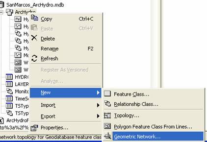
Right Click on the ArcHydro feature dataset and select New / Geometric Network.� You have to have ArcInfo to complete this task � ArcView does not create networks.��
Click Next on the Geometric Network Wizard options until you get to Selecting the feature classes and network name.� Select HydroEdge and HydroJunction as your network feature classes.� Change the network name to HydroNetwork.�
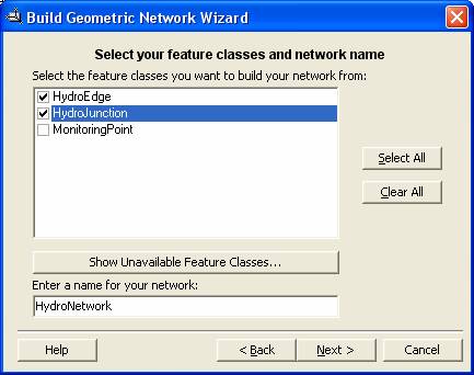
Continue through the wizard and accept all the defaults EXCEPT say yes when it asks if you want complex edges in the network.� When you finish you�ll see that you�ve created a new geometric network, HydroNetwork, which includes a set of generic network junctions called HydroNetwork_Junctions whose function is to provide geometric connectivity between the HydroEdge features.��

Close ArcCatalog, open ArcMap and display the new network.
Notice that when you add the network, the HydroEdge, HydroJunction, and HydroNetwork_Junction feature classes are added to the map.� The HydroJunction features which represent MonitoringPoints are now part of the HydroNetwork.� This is be very useful when we do flow tracing, which we are going to do next!
The Utility Network Analyst is an extension to ArcMap for performing analysis with geometric networks. It is called the Utility Network Analyst because geometric networks in ArcGIS are most commonly used in the utility industry, but they are also helpful in water resources research.
Use View/Toolbars, to display the Utility Network Analyst toolbar and select Flow/Display Arrows.� You�ll see that there are set of * symbols displayed, which means that there is no flow direction set on this network.��

ArcGIS has four possible values for flow direction along a
line: 0 = Uninitialized, 1 = WithDigitized, 2 = AgainstDigitized and 3 =
Indeterminate.�� These values refer to
the direction in which the line has been digitized (as shown by the order of
its vertices).�� Usually, the NHD lines
have been digitized from upstream to downstream, so the flow direction is set
to be WithDigitized.� The NHDinGeo geodatabase design has adopted
this convention from the Arc Hydro design.��
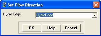
To apply the flow direction attribute values to the network, use the Arc Hydro tools Set Flow Direction (not Store Flow Direction!)
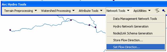
Choose HydroEdge in
the Set Flow Direction dialog, Press
Ok, and then press the set the flow direction according to the attribute FlowDir.
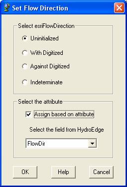
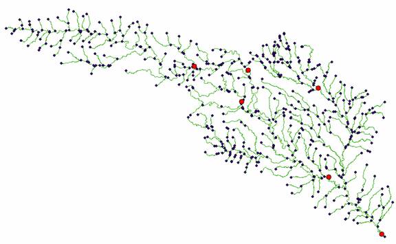
This action takes a couple of minutes as there are 557 Lines to be processed.
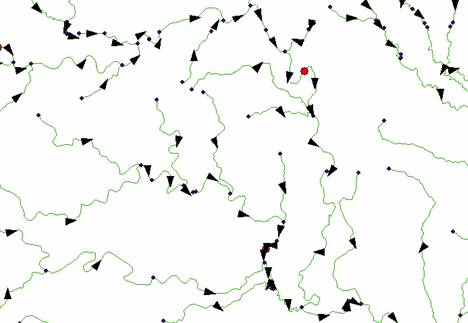
Now when we view the flow arrows, they will be pointing in the correct direction.
Once the flow direction is properly set, we can use the Utility Network Analyst to perform some flow tracing exercises.� Flow tracing works by placing flags on the network and tracing from a flag either upstream or downstream along the network.� Let�s try it.
Use the Add Junction Flag tool ![]() �on the Utility Network Analyst to place a flag
on the basins outlet junction.� This will
place a green square (representing a flag) on the junction.
�on the Utility Network Analyst to place a flag
on the basins outlet junction.� This will
place a green square (representing a flag) on the junction.
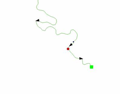
Set the Trace Task
to Trace Upstream.� ![]()
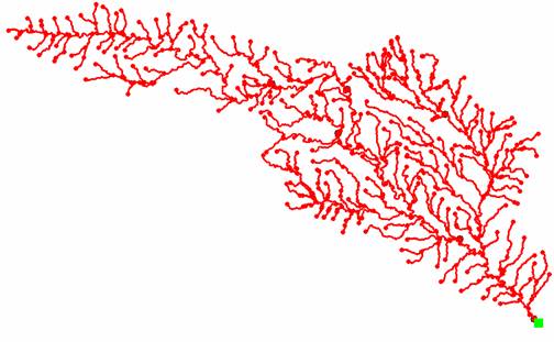
Now use the Solve tool
![]() �also on the Utility Network Analyst to run the
trace upstream process.
�also on the Utility Network Analyst to run the
trace upstream process.
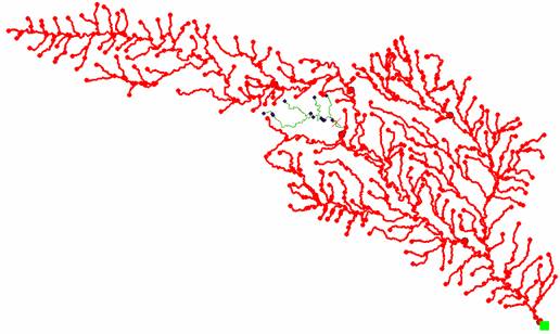
This procedure will turn the entire network red indicating that all reaches are upstream of the outlet junction (as we would expect).� This is a very useful thing to do when building you own networks because it insures that the network is properly �hooked-up�.
In addition to junctions, the Utility Network Analyst also allows you to place barriers along the network to block a tracing path.�
To clear the results of the previous run, select Analysis/Clear Results.� You can also clear flags and barriers here.�
Place an edge barrier ![]() �(the tool is under the junction flag tool) on one of the reaches and try to
upstream trace again.���
�(the tool is under the junction flag tool) on one of the reaches and try to
upstream trace again.���
The Utility Network Analyst can also do actual feature selections.� Suppose we wanted to select all the downstream edges and junctions for a particular place on the network.
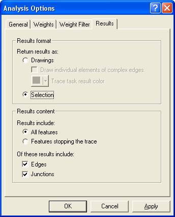
First, open the Options window Analysis/Options.� Under the Results tab, change the results format to Selection.�
 �
�
Next clear the flags, junctions, and barriers from our previous trace.
Place a flag on an edge in the network and press the Solve button.
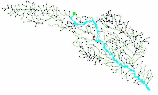
The analyst now selects the features instead of creating a red graphic over the features.�
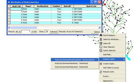
Open the HydroJunction feature class attribute table and notice that four of the six features were selected meaning that these four are downstream of the junction I traced from.�

We can get the monitoring points related to these features by selecting Options/Related Tables/HydroJunctionHasMonitoring Point:Monitoring Point.
This will bring up the MonitoringPoint attribute table with three of the 49 features selected.� These selected monitoring points are downstream of the junction I traced from.�
To be turned in:� Do a trace from the most upstream junction in
the network and �trace downstream� to the outlet.�� What is the total length (km) of the flow
path thus identified?
How many
HydroJunctions are selected?�� What
stream gages measure flow along this path (give the stream gage names and USGS
ID values).�� What is the total area of
the watersheds that this flow path traverses?
Arc Hydro has some other neat tools for determining networkwork attributes.� One of them finds the Length Downstream for Junctions.
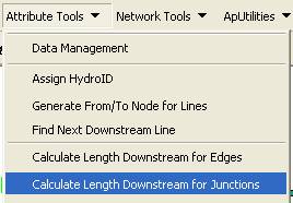
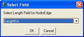
Invoke this tool and select HydroJunctions as the feature class to be processed

and select LengthKm as the field on HydroEdges to be used for the Length calculation
Now if you click on the HydroJunction for the stream gage of
the

and if you navigate through the + signs you can see the gage and the watershed that is relationally linked to this stream gage.
To be turned in:� What is the drainage area of DEM watershed
draining to the gage on the
That�s it for network analysis.� You can see how power these tools can be for a complex network where it is not immediately clear what is downstream of what.� This last process of finding the related time series recorded downstream of an arbitrary point on the network is a good segue into our next topic: visualizing space and time in ArcGIS.�
Viewing Temporal Data
in ArcGIS
Another useful task within ArcMap for utilizing ArcHydro is to simply visualize the spatial and temporal patterns of hydrologic phenomena (like rainfall or streamflow).� To do this, ESRI developed an extension for ArcMap called the Tracking Analyst.�
The Tracking Analyst is flexible in the format of data required and the options for symbolizing and rendering the spatial features according to the magnitude of their time series value for a given time-stamp.� The required information is a shape, a date, and a value (i.e. where, when, and what) that can be stored in one feature class or one feature class and one associated table.� This flexibility allows the Tracking Analyst to display features that move and/or change shape through time in addition to features that have time-indexed attribute values.� Below is a list of possible scenarios for features changing through space and over time:
� Stationary features with dynamic attribute (e.g. a stream flow gage)
� Stationary features with dynamic shape (e.g. an inundated river)
� Moving features with dynamic attribute (e.g. particle tracing in the subsurface)
� Moving features with dynamic shape (e.g. a hurricane)
Let�s get started with using Tracking Analyst ���
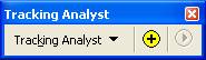
If the Tracking Analyst toolbar is not present on the ArcMap user interface, click View�Toolbars, and then select Tracking Analyst.� This displays the Tracking Analyst toolbar (shown below).�
Check to make sure the Tracking Analyst extension is selected (if not, the buttons on the Tracking Analyst will be disabled).� Click Tools�Extensions.� Click on the box next the �Tracking Analyst� if it is not already checked.
First we need to create an attribute in the MonitoringPoint feature class that distinguishes between streamflow and rainfall gages.
Open the MonitoringPoint feature class attribute table.� Select only the features with eight-digit HydroCodes.� These are the streamflow gages.� Right-click on the FType field and select Calculate Values.� Press Yes.�
In the Field Calculator window, make the FType = 1.� We are defining FType of 1 to mean a streamflow gage.

Repeat this same process for the remaining features and set their FType = 2.� We are defining FType of 2 to mean a rainfall gage.
�
You can now close the attribute table.
We will now create a Temporal Layer using the
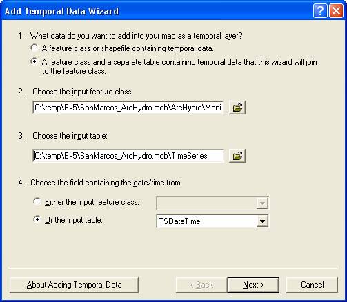
MonitoringPoint feature class and the TimeSeries table.� Click the ![]() �button on the Tracking Analyst toolbar.� Select the second option for the first
question (What data do you want to add into your map as a temporal layer),
browse to the input feature class (MonitoringPoint)
and then to the input table (TimeSeries).� Finally, select TSDateTime from the input table as the date/time field.� The form should look like what�s pictured
below.� Click Next.
�button on the Tracking Analyst toolbar.� Select the second option for the first
question (What data do you want to add into your map as a temporal layer),
browse to the input feature class (MonitoringPoint)
and then to the input table (TimeSeries).� Finally, select TSDateTime from the input table as the date/time field.� The form should look like what�s pictured
below.� Click Next.
On the next page, choose HydroID as the join field in the input feature class and FeatureID as the join field in the input table.� This will provide the link between features in the feature class and their associated time series records. Click Finish.� It should only take a second for ArcMap to generate the temporal layer named TimeSeries & MonitoringPoint.� Notice that this new layer is simply the MonitoringPoint features joined to TimeSeries time series table.� Open up the layer�s attribute table to take a look.
If you open the attribute table for the new temporal layer TimeSeries & MonitoringPoint,
you�ll see a table with 627 features, one representing each time series record
for each feature.� We�ll now symbolize
this layer to show the storms movement over the
But before we continue, recall that the MonitoringPoint feature class has both streamflow and rain gages.� We need to use a definition query so that the layer only shows the rainfall gages.� Then we�ll repeat this process to create a temporal layer for the stream flow gage.
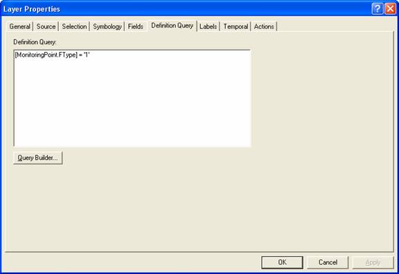
In the TimeSeries & MonitoringPoint layer properties, select the Definition Query tab.� Type [MonitoringPoint.FType] = 1 into the text box (you could also use the Query Builder button).� This will limit the temporal layer to showing only streamflow gages.
Now let�s symbolize the data.� Select the Symbology tab in the Layer Properties form.�
You�ll notice that the symbology tab for at temporal layer is somewhat different than one for a normal spatial layer.� In the top left corner in the Show box there are three options.� The Events option controls how the features are symbolized for each time step.� The Time Window option allows you to change the event symbology as time progresses.� The Tracks option can be used to connect features as they move through time (i.e. to show the path of an airplane as it moves).��
To symbolize the
Events:
Make sure the Events option is highlighted in the Show box.� In the Drawn As box, select Graduated symbols under the Quantities heading.�� For the Fields value, select TimeSeries.TSValue as the value (see figure below).�
Click the Classify button and chose to classify the values into 4 Quantiles.�
Color the symbols appropriately (I used no color for 0 rain and dark blue for largest category of rain).

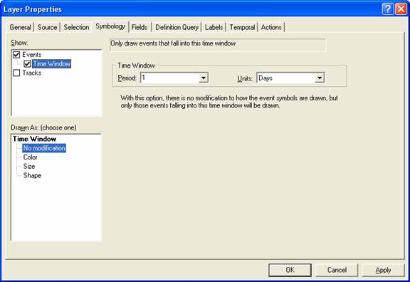
To set a Time Window:
In the Show box of the Symbology tab, check the box next to Time Window.� With Time Window highlighted, choose to limit the display of data to a one day time window.
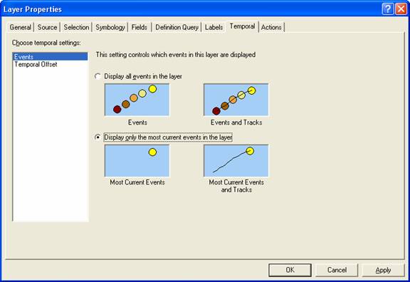
Finally, on the Temporal tab, select to show only the most current events.
Close the Layer Properties form.
You have now symbolized the temporal layer for rainfall and are ready to animate the rainfall over time.�
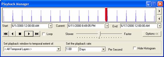
Press the ![]() �button on the Tracking Analyst toolbar.� This will launch the Playback Manager (shown
below).� Click Options and set the playback rate to 1 day.� You can press the play button to start the
animation, or just move the red bar to the right.� Try both.�
�button on the Tracking Analyst toolbar.� This will launch the Playback Manager (shown
below).� Click Options and set the playback rate to 1 day.� You can press the play button to start the
animation, or just move the red bar to the right.� Try both.�
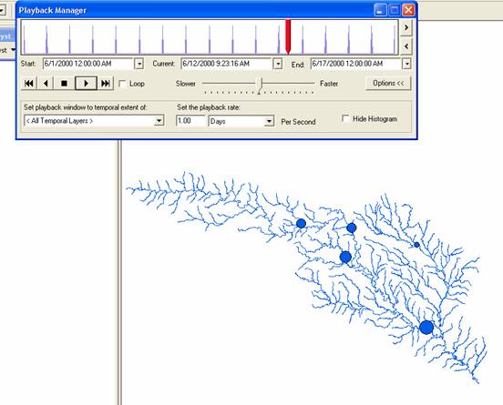
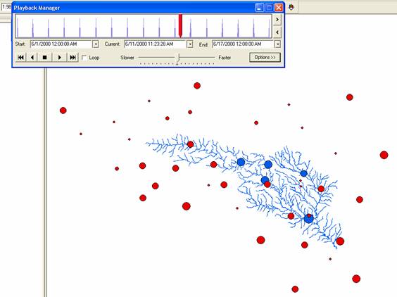
We can see that there was a large storm event during this
period with peak flow of over 800 cfs averaged over a day.� To see how this rain event affected
streamflow, we�ll follow the same procedure outlined above to add a second
temporal layer for the rainfall gages in the
Create a second temporal layer following the same procedure, except this time instead of having the definition be [MonitoringPoint.FType] =2 (for rainfall), instead use [MonitoringPoint.FType] = 1.� When you�re done, you should be able to view the rainfall event and the resulting increase in stream flow.��
Tracking Analyst can also be used to make a movie.� The movie can then be put into PowerPoint or on the web and act as a power visualization tool.
On the Tracking Analyst toolbar, press Tracking Analyst �
Animation Tool.� Keep the
While having the rainfall data geospatially reference by the Hydrologic Response Units (or the NEXRAD cells) is useful, potentially more useful is having the data geospatially referenced by the catchments.� This is a first step in using the rainfall to estimate streamflow.� We�ll do this another time!
To be turned in:� Graph rainfall and streamflow a few of the
gaging stations.� Did you notice that one
streamflow gage on the
Ok, you�re done!
Summary of items to
be turned in:
(1)� A screen capture of the attribute table of
the StreamGageAddressPoint feature class and a screen capture showing one of
the USGS gages with its corresponding stream address point located on the
stream line.
(2)� Do a trace from the most upstream junction in
the network and �trace downstream� to the outlet.�� What is the total length (km) of the flow
path thus identified?
How many
HydroJunctions are selected?�� What
stream gages measure flow along this path (give the stream gage names and USGS
ID values).�� What is the total area of
the watersheds that this flow path traverses?
(3)� What is the drainage area of DEM watershed
draining to the
(4)� Graph rainfall and streamflow a few of the
gaging stations.� Did you notice that one
streamflow gage on the