Exercise 3: Map Projections and Coordinate Systems
CE 394K GIS in Water Resources
University of Texas at Austin
Fall 2001
Prepared by Kristina Schneider and David R. Maidment
Contents
Projections of the United States
Doing Projection in ArcToolbox
|
Step 1 |
||
|
|
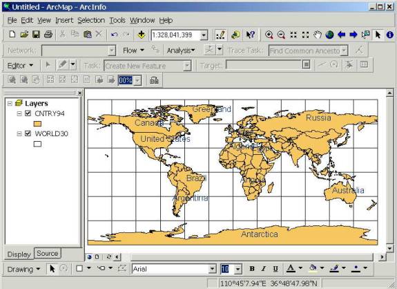
The files for this exercise are contained in the directory /class/maidment/giswr/mapproj in the LRC server. They are also available at ftp.crwr.utexas.edu in /outgoing/maidment/gisclass/mapproj as a zip file called mapproj. You can also download this file directly from this CD by clicking on mapproj.zip. These data are built into a geodatabase called Mapproj.mdb which contains four feature datasets: World: containing feature classes Cntry94 and World30 - countries and 30� meridians and parallels for the earth USA: containing feature classes States, Counties and Latlong - States and Counties of the US and a 5� grid of meridians and parallels Texas: containing Quad75 and Onedegtx - a coverage of Texas showing a 1� grid and 7.5' quad map extents Austin: containing Juris, Lakes, Roads - administrative boundaries of legal jurisdiction, lakes and roads in Austin, Texas. All these feature datasets contain data in geographic coordinates defined on the NAD83 datum. Download or link to these files now. 1. Start ArcMap. Click Add layers button You want to make the layer World30 rectangles show just their outlines, so they can serve as the coordinate system, using their 30 degree mesh. 2. Right-click on the World30 layer and click Properties. Navigate to the Symbology tab and double click on Symbol to get the Symbol Selector window. Select the Hollow color and press OK. You should see the World in Geographic Coordinates. 3. Right-click on the Cntry94 layer and choose Label Features. You�ll see that the countries are named.�� If you don�t like the font and color of the label, right-click on the layer and select Properties. Navigate to the Label tab and press the Symbol button. Here you can choose the font, color, and style you would prefer. This option labels all the features in the layer.��� If you want to label the features using another attribute besides the country name, you can also do that using the Label Properties window. 4. To label just a few features, first right click on the Cntry94 layer and deselect Label Features. On the Draw Toolbar there is a Label button that allows you to label individual features.�� It is found underneath the big A symbol shown below: Double click on the label button and keep the selections chosen by the computer.� Close the screen just opened and click on the countries you would like to label.� Be sure to have the Cntry94 feature class as the uppermost one in your legend, or you will get just numbers of the World30 boxes when you try to click on the countries to label them with names.�� Pretty cool!! Move the cursor around on the view and you will see a pair of numbers
above the view on the toolbar to the right of "scale" that alter as
you move the cursor. These give the location of the cursor and from the
values displayed you can see that these data are Latitude and Longitude displayed
in Degrees, Minutes and Seconds. 5. Save the Map file as World.mxd Questions:
|
|
|
Step 2 |
The World in Robinson Projection |
|
|
|
The actual projection of the layers cntry94 and World30 is geographic, however these layers can be viewed in different projection systems. A common projection system for the World is the Robinson projection. 1. Create new Data Frame, using Insert/New Data Frame.� Select View/Data Frame Properties� Select the General tab and name the data frame Robinson.� Right click on the World30 feature class in Layers, select Copy, then Right click on the Robinson data frame and select Paste Layer.�� You�ll see the World30 feature class symbol appear in the Robinson data frame.�� Do the same for the Cntry94 feature class.� Right click on the Robinson data frame and select Activate to display the data in this frame.�� Pretty cool!�� To copy the two feature classes as a group, you can right click on a data frame in the table of contents (with Display tab active) and create a new Group Layer. Then individual layers can be dragged and dropped onto the new Group Layer. Then the entire group layer can be copied and pasted between data frames.
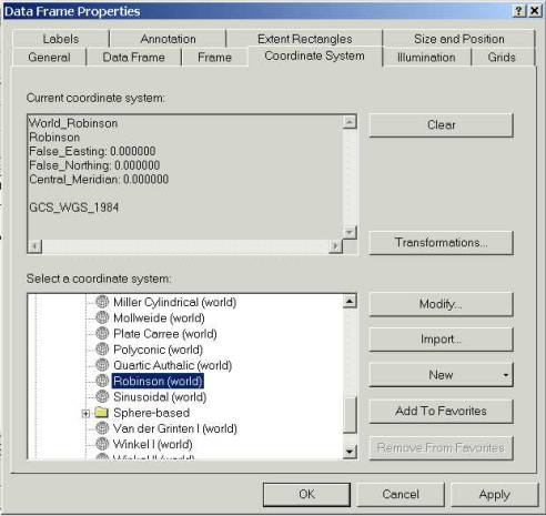
2. Right click on the Robinson data frame, and select the Coordinate System tab. Under the Select a Coordinate System box, choose the Predefined folder. Then select Projected Coordinate Systems/World/Robinson.�� Click OK. A warning may appear but we can ignore it for our purposes, so just click Yes. Ignore this message every time it appears throughout the exercise. You will see the World appear in a Robinson projection. The files themselves have not been projected permanently but are only displayed in the new projection.��
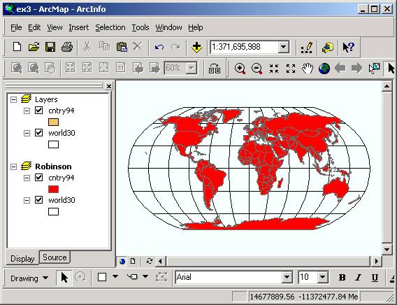
The Robinson projection is a relatively new map projection for the earth designed to present the whole earth with a minimum of distortion at any location. If you move the cursor over this space, you'll see that the coordinates are now in a very different set of units, meters in the projected coordinate system. 3. Play with the different projections and explore the different shapes the world can take.�� Note that the data frame showing in the Data View is the one most recently created.�� If you want to view another data frame, Right click on the data frame name, and choose Activate.� You can create a layout that contains several different data frames.�� Switch to the Layout view, and
you�ll see both data frames displayed. To be turned in: a Layout showing the World in Geographic Coordinates, in Robinson Projection, and a projection of your choosing.
|
|
|
Step 3 |
|
|
|
|
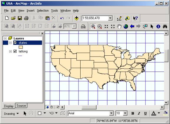
You will now examine map projections used for the continental United States. �� We could continue adding data frames to the previous map file, but to simplify things, lets create a new map file.� Use File/New/Blank document to create a new map file.�� Save the map file as USA.mxd. 1. Add the States and Latlong feature classes from the USA
feature dataset of mapproj.mdb.�
Click on the Zoom in tool
Questions:
|
|
|
Step 4 |
United States in Albers Equal Area Projection |
|
|
|
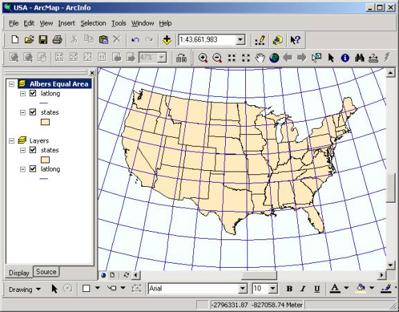
The Albers Equal Area projection has the property that the area bounded by any pair of parallels and meridians is exactly reproduced between the image of those parallels and meridians in the projected domain. That is, the projection preserves the correct area of the earth although it distorts the direction, distance and shape somewhat. 1. Create a new Data Frame and copy and paste in the layers Latlong and States from the previous frame. To copy the layers you must make the old data frame active by right-clicking on the frame and selecting Activated. Then to Paste the layers you must make the new frame active in the same manner. 2. Rename the data frame as Albers Equal Area.� Double Click on the data frame and go to the Coordinate System tab. Select the coordinate system Predefined/Projected Coordinate System/Continental/North America/USA Contiguous Albers Equal Area Conic projection.� Zoom into the US without Alaska.
3. Compare the United States in geographic coordinates and in the Albers projection. You will see that in geographic coordinates the United States appears to be wider and flatter than it does in Albers Equal-Area Projection. This does not occur because Canada is sitting on the USA and squishing us! This effect occurs because as you go northward, the meridians converge toward one another while the successive parallels remain parallel to one another. When you reach the north pole, the meridians converge completely. If you take a 5 degree box of latitude and longitude, such as one of those shown in the views, the ratio of the East-West distance between meridians to the North-South distance between parallels is Cos (latitude): 1. For example, at 30�N, Cos(30�) = 0.866, so the ratio is 0.866 : 1, at 45�N, Cos(45�) = 0.707, so the ratio is 0.707 : 1. In the projected Albers Equal Area frame the result is that square boxes of latitude - longitude appear as elongated quadrilaterals with a bottom edge than their top edge. In geographic coordinates, the effect of the real convergence of the meridians is lost because the latitude and longitude grid form a set of perpendicular lines, which is what makes the United States seem wider and flatter in geographic coordinates. 5. Save the USA.mxd project. To be turned in: a Layout showing the United States in Geographic Coordinates and in the Albers Equal Area projection. |
|
|
Step 5 |
|
|
|
|
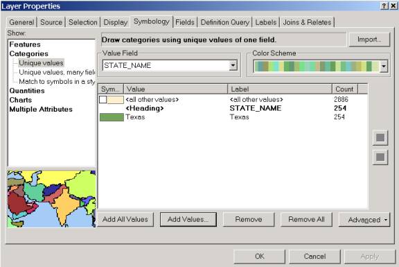
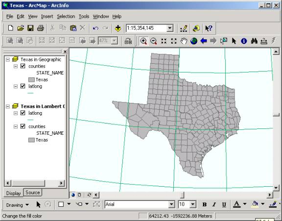
You will now examine the effect of various map projections up a map of the State of Texas. 1. Create a new map document, Texas.mxd.�� Add in the feature classes Counties and latlong from the USA feature dataset of the mapproj.mdb geodatabase. The feature class Counties is a counties layer of the United States, including Alaska and Hawaii. Rename the Layers data frame Texas in Geographic. 2. To make it easier to determine the counties located in Texas, go to the Counties / Properties and then to the Symbology tab. Choose to display the Counties by Categories with the Unique value of State_Name. Press the Add Values� button (don�t choose Add All Values!)� and select Texas pressing OK. Deselect the check mark for <all other values>, which will leave only counties with the state_name as Texas to be shown.
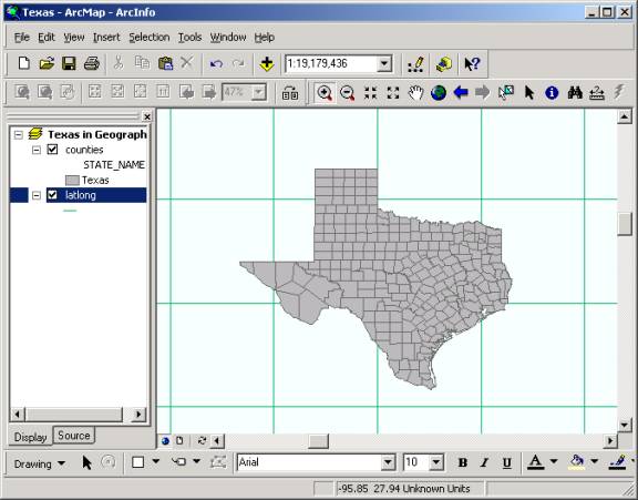
3. Click OK, and you will see only the counties in Texas remain in the view. Zoom in to see the larger view of Texas counties.
The latitude/longitude grid displayed is at 5-degree intervals of latitude and longitude. You can determine what latitude or longitude a particular line represents by moving the cursor to any line and read the latitude and longitude number displayed on the right corner of the tool bar. Questions:
|
|
|
Step 6 |
Texas in Lambert Conformal Conic projection |
|
|
|
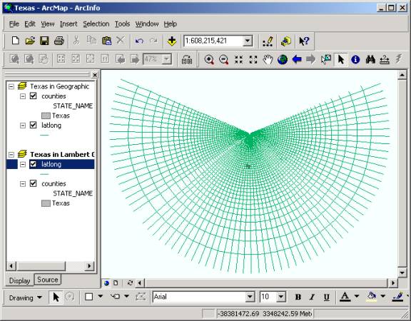
The Lambert Conformal Conic projection is a standard projection for presenting maps of land areas whose East-West extent is large compared with their North-South extent. This projection is "conformal" in the sense that lines of latitude and longitude, which are perpendicular to one another on the earth's surface, are also perpendicular to one another in the projected domain. 1. Create a new data frame, copy and paste Latlong and Counties to it from the previous view. Choose Properties for the data frame, rename the data frame as TX in Lambert projection. 2. Move to the Coordinate System tab and select Predefined/Projected Coordinate System/Continental/North America/USA Contiguous Lambert Conformal Conic projection. Click OK. Notice how the meridians now fan out from an origin at the center of rotation of the earth (a consequence of using a conic projection centered on the axis of rotation of the earth). The display shown is that produced by cutting the cone up the backside and unfolding the cone so that it lays flat on the table.
3. Zoom in to see the detailed Texas Counties in Lambert Conformal Conic projection.
Notice that Texas appears to be tilted to the right slightly. This occurs because the Central Meridian of the projection used is 96�W, which would appear as a vertical line in the display if it were shown. Regions to the West of this meridian (most of Texas) appear tilted to the right while those to the East of this meridian appear tilted to the left. |
|
|
Step 7 |
Texas in the Texas Centric Mapping System |
|
|
|
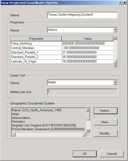
In order to present a pleasing map of Texas, and to minimize distortion of distance in State-wide maps, the Texas State GIS Committee, has approved a standard projection of Texas called the Texas Centric Mapping System (see http://tgic.state.tx.us/standards/tgic-s06.doc for details. There are two variations on this projection, one in Lambert Conformal Conic coordinates and the other in Albers Equal Area coordinates. We�ll use the Albers Equal Area version since that works best for water resources computations that require true earth area to be preserved in map projections. The definition of this projection is: Datum: North American Datum of 1983 (NAD83) This means the standard parallels where the cone cuts the earth's surface are located at about 1/6 of the distance from the top and bottom of the State, respectively, and that the origin of the coordinate system (at the intersection of the Central Meridian and the Reference Latitude) is to the South of Texas in the Gulf of Mexico, to which the coordinates (x, y) = (1500000, 6000000) meters is assigned so that the (x, y) coordinates of all locations in the State will be positive. 1. Create a new data frame, copy and paste Latlong and Counties to it from the previous view.� Double-click on the data frame name and rename it Texas Centric 35.0. Click on the Coordinate System tab. With the <custom> folder highlighted select the New� button on the right to create a new Projected Coordinate System. Fill out the parameters with the values given above.�� You also have to select a Geographic Coordinate System to specify the earth datum.� Select North American/North American Datum 1983.
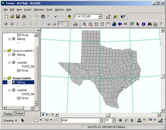
2. Click both OKs in the two dialog box and you'll see the map of Texas transformed to a nice upright appearance, the Texas Centric Mapping System. Zoom into the state of Texas.
|
|
|
Step 8 |
Texas in Universal Transverse Mercator (UTM) Projection |
|
|
|
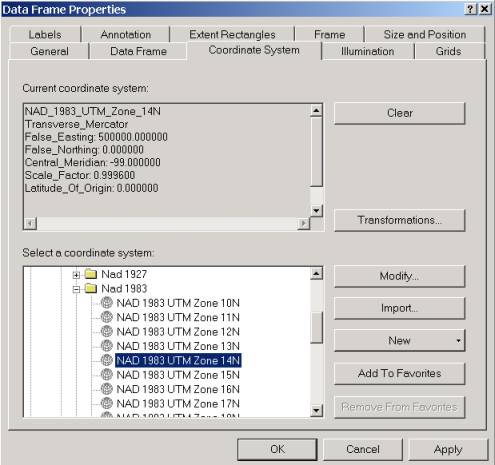
The Universal Transverse Mercator projection is actually a family of projections, each having in common the fact that they are Transverse Mercator projections produced by folding a horizontal cylinder around the earth. The term transverse arises from the fact that the axis of the cylinder is perpendicular or transverse to the axis of rotation of the earth. In the Universal Transverse Mercator coordinate system, the earth is divided into 60 zones, each 6� of longitude in width, and the Transverse Mercator projection is applied to each zone along its centerline, that is, the cylinder touches the earth's surface along the midline of each zone so that no point in a given zone is more than 3� from the location where earth distance is truly preserved. 1. Create a new data frame, copy and paste Latlong and Counties to it from the previous view.� Double-click on the data frame name and rename it UTM Zone 14N. Click on the Coordinate System tab and select Predefined/Projected Coordinate System/Utm/Nad 1983/NAD 1983 UTM Zone 14N projection.
These parameters mean that the Central Meridian of Zone 14 is at 99�W so that it covers from 96�W to 102�W; the Reference Latitude is 0.0000 (the equator, which is 0�N); the origin of the coordinate system is at the intersection of the Central Meridian with the Reference Latitude and thus is at (0�N, 99�W), where the coordinates are (x, y) = (500,000, 0) m. The false Easting of 500,000m is to ensure that all points in the zone have positive x coordinates. The y-coordinates are always positive in the Northern hemisphere because 0 is at the equator. In the Southern Hemisphere, a false Northing of 10,000,000m is applied to ensure that the y-coordinate is always positive. The Scale Factor of 0.9996 means that along the Central Meridian, the true scale of 1.0 is reduced slightly so that at locations off the true meridian the scale factor will be more nearly 1.0 (the Transverse Mercator projection distorts distance positively as you move away from the Central Meridian). 2. Click both OKs to see the projection applied. The pattern of meridians and parallels looks strange, converging at top and bottom of the picture, which correspond to the North and South Poles, respectively. 3. Zoom in on Texas, the map of the State looks much as it did in the Texas State Mapping System using the Lambert Conformal Conic projection. 4. Save the Texas.mxd Map document. Questions: To be turned in: A Layout showing Texas in Geographic,
Lambert Conformal Conic, Texas Centric and UTM projections |
|
|
Step 9 |
|
|
|
|
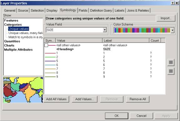
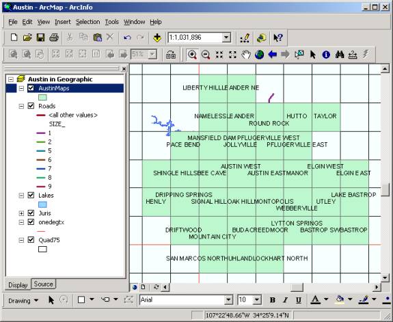
You have viewed the effect of different projections on different scales from the World, Country and State level. In the next few steps, you will take a look at the City of Austin and the effect of two map projections upon a map of the City. 1. Create a new map document, Austin.mxd, and add in the layers Juris, Lakes, Roads from the Austin feature dataset, and Quad75, and Onedegtx from the Texas feature dataset in the Mapproj.mdb geodatabase.� The feature class Juris is a coverage of the legal jurisdictions of the City of Austin. The classes Lakes and Roads are coverages of the lakes and main roads of the Austin area respectively. The layer Quad75 is a mesh of 7.5 minute quadrangles for Texas with map sheet names in each quad, and the layer Onedegtx is a line layer with lines each one degree of latitude and longitude so you can see where Austin is located geographically. All these layers are in geographic coordinates, NAD83 datum. 2. Double-click on the data frame name and rename it as Austin in Geographic. 3. Right-Click on the Juris layer and select Zoom to Layer. Drag the Roads and Lakes above the Juris layer. Drag the Onedegtx layer down to just above the Quad75 layer, and make Quad75 Hollow, with only outline. (See instructions in Step 1).�� Symbolize Onedegtx using the Highway color (Red, size 3). You can get a better picture of Austin by using the Symbology tab on the Roads layer to classify the roads by Size (Size = 1 is the largest road for IH-35 and the Mopac expressway), and on the Juris layer by Name. The names give the locations of surrounding cities and 2 mile and 5 mile buffer zones around the Austin City Limits called Extra Territorial Jurisdictions, or ETJ's. 4. Right-click on Roads layer and select Properties, navigate to Symbology. Select to represent the layer with a Unique Category with SIZE in the Value field. Use an appropriate color scheme.�� To make the lines thicker, click on the all other values line, to bring up the Symbol Selector window, set the Width to 2.00, and then reclick on Add all Values in the Layer Properties window to resize all the lines to size 2.�
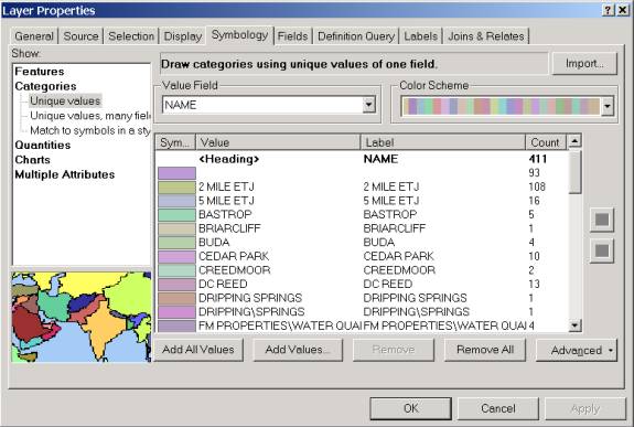
5. Click OK. 6. Repeat this process with the Juris layer placing Name in the Value field. Change the Color Schemes to Pastels.
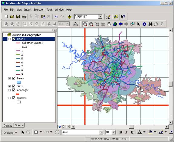
7. Click Ok. You will see the City of Austin classified by legal jurisdictions and the City of Austin in Geographic Coordinates.
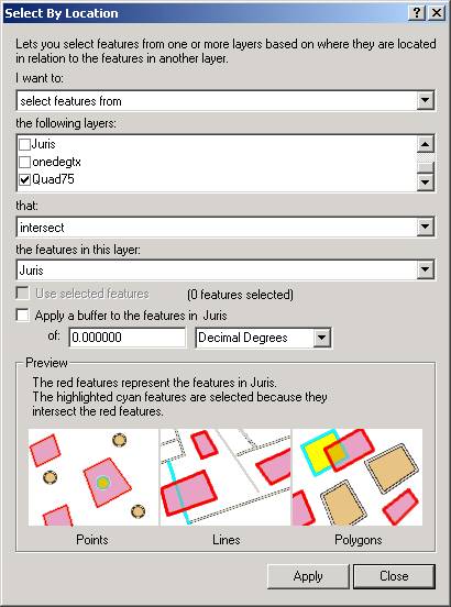
8. The Quad75 layer is the 7.5 Minute Quadrangle Sheet Coverage. Right-click on the 75Quad layer and select Zoom to Layer so that you see all of Texas displayed in 7.5 min quadrangle sheets. � Resize the Onedegtx lines to size 1 so that they are not too dominant in the map.�� 9. To identify the map sheets needed to cover Austin, use Selection/Select by Location and fill the resulting window as below: Select feature from Quad75 that intersect Juris.� You�ll see a set of quadrangles selected on the map.
10.� Right click on Quad75, and select Data/Export Data name the resulting file AustinMaps.shp (make sure that it is saved outside your Mapproj.mxd), and add it to the display.�� Right click on AustinMaps and select Label features to show the map names.�� You can open the attribute table of this file AustinMaps.dbf in Excel and select the list of map names.
Questions: To be turned in: Make a list of the names of the 1:24,000 scale map sheets (7.5' quads) that are needed to cover Austin. |
|
|
Step 10 |
Austin in State Plane - 1927 Projection |
|
|
|
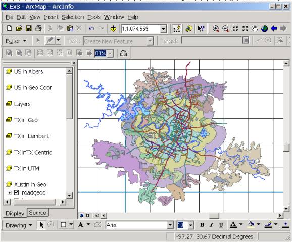
The State Plane - 1927 projection is a standardized projection that is used for definition of legal boundaries in Austin. Texas has five zones in the State Plane coordinate system, each defined using the Lambert Conformal Conic projection, with different projection parameters depending on which zone you are in. Austin is in the Texas Central Zone. The 1927 refers to the North American Datum (NAD) 27 datum. 1. Create a new data frame, load Juris, Lake, Road, Quad75, and Onedegtx from the geodatabase.� Double-click on the data frame name and rename it Austin in State Plane. Click on the Coordinate System tab and select Predefined/Projected Coordinate System/State Plane/NAD 1927/NAD 1927 Stateplane Texas Central FIPS 4203 projection. Click OK. 2. Right-click on Juris and select Zoom to layer. Play with the Symbology until it looks similar to the Austin in Geo data frame.
To be turned in: A Layout showing Austin in Geographic coordinates and in State Plane Coordinates. |
|
|
Step 11 |
|
|
|
|
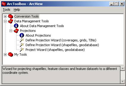
Up until now we have changed the projection of the data frame but not the actual projections of the shapefiles. Therefore, if you reopened each shapefile we worked with it would always appear in its original projection. File projection can be performed in ARC/INFO. However, ArcGIS offers the ArcToolbox program, which makes projection simpler.� 1. Save your Map document and close ArcMap. This is because we cannot work on the files we would like to project in ArcToolbox while they are in ArcMap. 2. Open ArcToolbox and navigate to the Projections toolkit located in Data Management Toolbox.�� This picture shows the range of tools available for projection in ArcView 8.1, which permits projection of shapefiles and feature classes.�
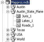
We are going to project the contents of the Austin feature dataset from geographic coordinates to State Plane coordinates. 3. Double click on the Project Wizard (shapefiles and geodatabases) and select the Austin feature dataset from the Mapproj.mdb geodatabase from the data directory. Press Next.� You�ll be prompted to select where the output feature dataset will be located.�� Call it Austin_State_Plane and browse to the Mapproj.mdb geodatabase to show where the new feature dataset will be stored.� Press the Select Coordinate System� button, then press the Select� button. This button will allow you to select a predefined coordinate system.. Navigate through the directories in this order Projected Coordinate System/State Plane/Nad 1983 (feet)/NAD StatePlane Texas Central FIPS 4203 (feet) and click Add. 4. Press OK and Next. The window will display the coordinate extents for the dataset. 5. Press the Next button to accept the default values given above. Press Finish and a status bar will show the progress of the projection. You�ve just projected all the feature classes in the Austin feature dataset to State Plane coordinates!!�� Pretty cool!! 6. Close ArcToolbox and open Arc Catalog, you�ll see that you�ve got a new feature dataset with copies of the three feature classes in the Austin feature dataset with a _1 added onto the name of each:
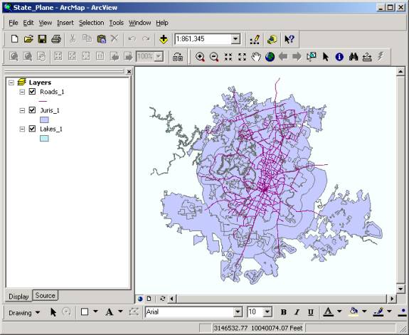
7.� Open a new ArcMap document.�� Add the contents of the Austin_State_Plane feature dataset.� Open the Properties of the data frame and change to name to projected. Then go to the Coordinate System tab and you will notice the projection is NAD_83_StatePlane_Texas_Central_FIPS_4203 (feet), as required.�� Pretty cool!!! � Notice the numbers in the lower right hand corner are not latitude and longitude any more. They are in the units of the State Plane coordinates - feet. Open the attribute table of the Juris, and navigate to the right hand end of the table.� You�ll see that two new fields have been created, Shape_Length and Shape_Area, which refer to the length (ft) of the perimeter and the area (ft2) of the polygon, for each feature in the Juris class. If you want, you can project the 7.5 quadrangle map, the roads, the lakes and the one degree boxes similarly, and add them to the new data frame. Verify that it looks the same as the Austin in State Plane data frame. Question: The area over which the City of Austin has "Full Purpose" jurisdiction is the area in the center of this map. The areas around this are areas in which the City has limited jurisdiction or areas, which lie within surrounding cities. Over what % of the area shown in the Juris polygons does the City of Austin have "Full Purpose" jurisdiction? Briefly explain how you got the answer. |
|
|
Step 13 |
1. Save your document in ArcMap. |
|
|
|
You're done!! |
|
Go to the Class Home Page