Exercise 2. Building a Base Map and a Point Shapefile
CE 394K GIS in Water Resources
University of Texas at Austin
Fall 2001
Prepared by Kristina Schneider and David R. Maidment
- Goals of the Exercise
- Computer and Data Requirements
- Procedure for the Assignment
- Get Stream and Watershed Data for Water Resource Region 12
- Selecting the Guadalupe Basin Watersheds
- Getting the Guadalupe River Reaches
- Creating and Projecting Point Shapefile of Stream Gages
- Add Attributes to the Point Shapefile
- Creating a Chart and Layout
- Overlaying the Edwards Aquifer
- Downloading USGS Flow Data
Goals of the Exercise
This exercise is intended for you to build a base map of geographic and flow data for a watershed using the Guadalupe Basin in South Texas as an example. This base map comprises watershed boundaries from the US Geological Survey's Hydrologic Unit Code (HUC) coverage and streams from the US Environmental Protection Agency's River Reach File 1 (RF1) coverage. In addition, you will create a point coverage (shapefile) of stream gage sites by inputting latitude and longitude values for the gages in an Excel table that will be added to ArcMap. The table will be used to create an XY Event from which the shapefile will be created. You will then link to the US Geological Survey's Real Time data website in Texas, download some streamflow data and make a plot of the flow hydrograph.
Computer and Data Requirements
To complete this exercise, you'll need to run ArcGIS 8.1 from a PC.
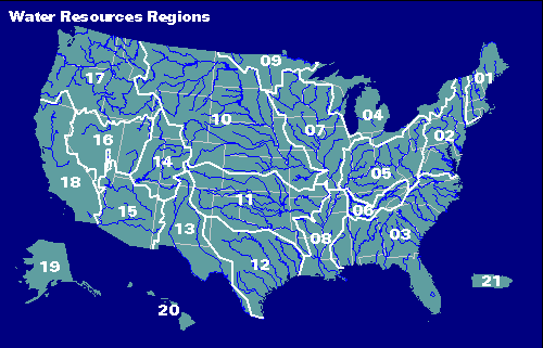
The HUC boundaries are a subdivision of the US made by the US Geological Survey to show major and minor river basins. There are 2-, 4-, 6-, and 8-digit HUC boundaries, where the larger the number is the smaller the area. The HUC8 boundaries are the basic ones.
The HUC and RF1 coverages for the United States can be downloaded over the internet:
Hydrologic Cataloging Unit
description http://water.usgs.gov/GIS/huc.html
Get the HUC coverages by 2-digit water resource region http://water.usgs.gov/lookup/getspatial?huc250k
Enhanced River Reach File 1
http://water.usgs.gov/lookup/getspatial?erf1
Get the RF1 data by two-digit water resource region ftp://water.usgs.gov/pub/dsdl/
It seems that using Wsftp to ftp://water.usgs.gov/pub/dsdl/ works a lot faster for downloading data than trying to do it through a web browser.
Procedure for the Assignment
Get Stream and Watershed Data for Water Resource Region 12
Logon to the computer of your choice and make a directory in your workspace for this exercise. I've saved the needed files in the class directory (Civil3/LRC/Class/Maidment/giswr/guadalupe/). The may also be downloaded as guadalupe.zip.
The files we'll use are:
Rf1_12.e00, huc12_250k.e00, edwards.shp, hucname.dbf, and rf1name.dbf
These files are in Arc/Info interchange file format, as indicated by the .e00 so you will need to import them using the Import from Interchange file tool in ArcToolbox.
- When you import rf1_12.e00, name the resulting coverage rf1reg12
- When you import huc_250k.e00, name the resulting coverage hucreg12
(1) Open ArcToolbox

(2) Select Conversion Tools/Import to Coverage/Import from Interchange File. Navigate to the location of the Input file. Then indicate where the output coverage should be located and what it should be called.
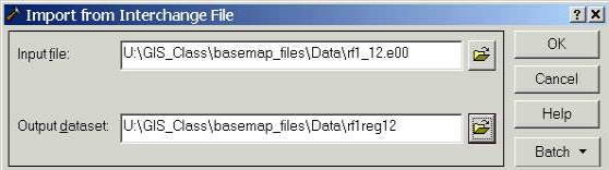
Press OK. Don't worry if processing takes a while, the file is rather large. (3) Repeat the process with the huc250k.eoo file.
Selecting the Guadalupe Basin Watersheds
The Hucreg12 and Rf1reg12 coverages cover a large region and we only want to work in the Guadalupe Basin. We'll use ArcMap to identify which HUC's cover the Guadalupe Basin and to create new shapefiles of these portions of the coverages.
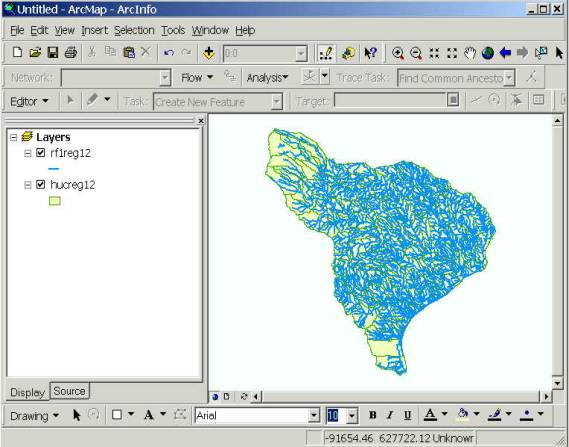
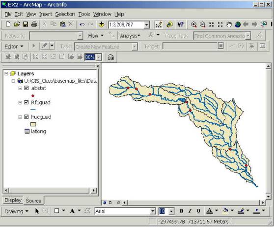
(1) Start up ArcMap and add the hucreg12 polygon theme and the rf1reg12 line theme to your map. Recolor the theme as necessary. These are ArcInfo coverages and to make them easier to work with, we’ll convert them to shape files. (2) Right click on each of the two themes in turn, and using the command Data/Export Data . . . to make a new copy of the data in shapefile format. Save the shapefiles in your working directory and give them the same names as the coverages (Hucreg12.shp, Rf1reg12.shp). You will be asked if you would like to add the exported data to the map as a layer, answer Yes. Right Click on the coverages and select Remove to delete the two coverage themes you began with. If you make a mistake later in the exercise, you can reconvert the coverages to shapefiles and start over.
(3) Save the ArcMap file as ex2.mxd.
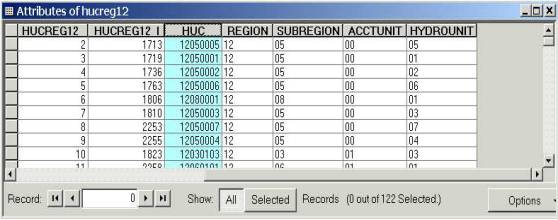
(4) Right click on the hucreg12 theme and select Open Attribute Table to bring up the table of its attributes. Scroll across the fields and see the Hydrologic Unit Code (HUC ), Region (first 2 digits of HUC), Subregion (second 2 digits of HUC), Basin (third 2 digits of HUC) and the Subbasin (fourth 2 digits of HUC).
You’ll see that these huc watersheds are identified by numbers rather than names. I have a separate names file hucname.dbf that I prepared from another HUC coverage.
(5) Hit the Add Data button ![]() and in the dialog box that appears, select
the hucname.dbf table. The table hucname is added to your map. We’ll join this table to the Huc
attributes so that we can identify the Huc watersheds by name.
and in the dialog box that appears, select
the hucname.dbf table. The table hucname is added to your map. We’ll join this table to the Huc
attributes so that we can identify the Huc watersheds by name.
(6) Right Click on the hucreg12 layer and select Joins and Relates/Join.... What you are doing here is associating corresponding records in the two tables using Huc as the key field values that they have in common.
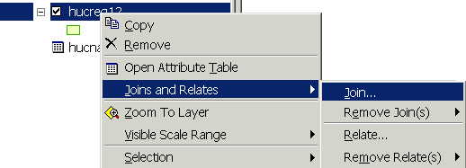
(7) Select the attribute HUC for question 1. For the second question, browse for the hucname.dbf table since it is not a layer in the map and therefore will not be automatically recognized. Again, for the third question select the HUC attribute. Click OK.
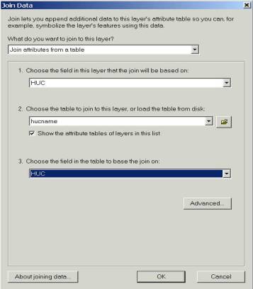
Voila!! Now we have a Name attribute on the Attributes of Hucreg12 table so that its easier to understand what river basin we are in.

Lets recolor the HUC’s by subregion to get some sense of the river basin organization within Region 12. You do this using the Symbology tab under layer Properties. Right Click on the layer and select Properties. Under Show in the same box choose select Categories/Unique Values, select hucreg12.SUBREGION as the value field to be symbolized, press Apply. Finally, press add all values.
If you use the Information tool ![]() you can click around and get a sense of the
names of the river basins and their subunits.
(8) Use the Select button
you can click around and get a sense of the
names of the river basins and their subunits.
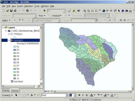
(8) Use the Select button ![]() and visually select the 4 huc units in the
Guadalupe basin. Hold down the shift
key so that you can select more than one at a time. Open the layer attribute table and press the Selected button.
This will show you the items you have selected. You will see that the Guadalupe
Basin is comprised of four sub-basins, the Upper [huc=12100201] , Middle [huc =
12100202] and Lower Guadalupe [huc = 12100204]basins and the San Marcos basin
[huc = 12100203]
and visually select the 4 huc units in the
Guadalupe basin. Hold down the shift
key so that you can select more than one at a time. Open the layer attribute table and press the Selected button.
This will show you the items you have selected. You will see that the Guadalupe
Basin is comprised of four sub-basins, the Upper [huc=12100201] , Middle [huc =
12100202] and Lower Guadalupe [huc = 12100204]basins and the San Marcos basin
[huc = 12100203]

(9) Right Click on hucreg12 and select Data/Export Data ... to produce a new theme. Name this theme hucguad.shp and save it in your local workspace for this exercise. The program with automatically convert only the selected features. You will be prompted to whether add this theme to the Map, click Yes. Notice the hucguad shapefile looks identical to the earlier hucreg12 theme selection for the Guadalupe basin. But the new hucguad shape file is much smaller. Notice that it carries all the attributes of hucreg12.shp and the hucname.dbf table that you joined before making the data export.
(10) Use Selection/Clear Selected Features to clear the selections you made from Hucreg12.shp.
Getting the Guadalupe River Reaches
Now we need to select the rivers in rf1reg12 that fall within the Guadalupe Basin. First, lets give the rivers some names.
(1) Right Click on the rf1reg12 layer and select Joins and Relates/Join. Select the field RR (River Reach) for question 1. For the second question, browse for rf1name.dbf table since it is not a layer in the map and therefore will not be automatically recognized. Again, for the third question select the RR attribute. Click OK.
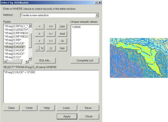
(2) Open the attribute table for the rf1reg12 table. Click on the Options/Select by Attribute and a dialog will appear. Use the Create a new selection Method and double click on the "rf1reg12.HUC6" field. Set this field equal to 121002. You'll see that now only the rivers within the Guadalupe River basin are selected. Notice that you are here selecting features using a query on tabular attributes, whereas in the previous section, you selected features using a graphical query on the map.
(3) Right Click on rf1reg12 and select Data/Export Data ... to produce a new theme. Name this theme Rf1guad.shp and save it in your local workspace for this exercise. You will be prompted to whether add this theme to the Map, click Yes.
(4) Highlight the hucreg12 and rf1reg12 themes in the legend bar (use Shift when highlighting the second theme). Right click an press Remove to delete them from the Map. From now on, we'll work with the Rf1guad and the Hucguad shapefiles to save time in displaying the themes.
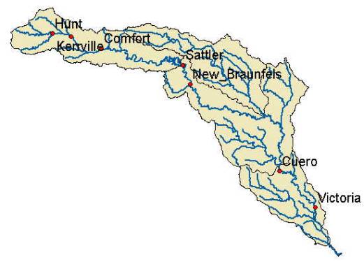
(5) Once you've got the Guadalupe Basin displayed, you can right click on the hucguad layer and select Zoom to layer to bring the Guadalupe Basin up to the full extent of the screen. Now you should be able to see the Guadalupe River Basin with all of its major river reaches.
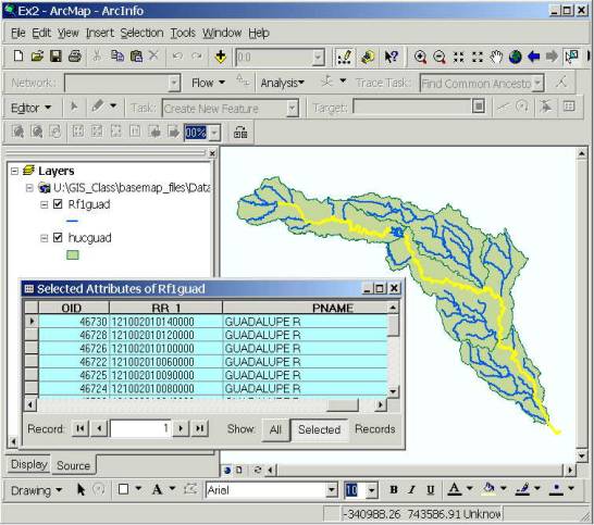
(6) Open the rf1guad attribute theme. Scroll across to the names of the rivers. Pname is the name of the river segment. Use the Select by Attributes interface to select "PNAME" = 'GUADALUPE R' and change the table view to the selected records. This shows the main channel of the Guadalupe River. The small gap in the center of the basin is the segment where the Guadalupe River flows through Canyon Lake, which is separately identified in the Pname field.
(7) Right click on the Rf1guad.shp theme and use Data/Export Data to export a new shape file of the Guadalupe River, called guadriver.shp, and at that to your map.
(8) Click on the symbol boxes to recolor your map to the form you want it in. Make a layout of this map, copy it to the clipboard and paste it to a Word file so you can turn it in.
To be turned in: the layout of the Guadalupe Basin streams and watersheds.
(7) Save your ArcMap document, ex2.mxd.
Creating Point Shapefile of Stream Gages
Now you are going to build a new coverage yourself of stream gage locations on the Guadalupe. I have extracted information from the USGS stream gage data books information about 7 gages on the main stem of the Guadalupe River (there are many other stream gages in this basin):
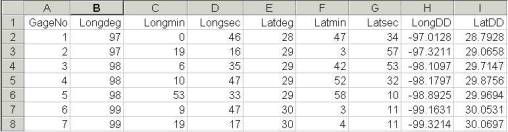
Seq# Station# Name Longitude Latitude Mean Annual Flow (cfs)1 08176500 Victoria 97 00 46 W 28 47 34 N 20952 08175800 Cuero 97 19 16 W 29 03 57 N 2094 3 08168500 New_Braunfels 98 06 35 W 29 42 53 N 552 4 08167800 Sattler 98 10 47 W 29 51 32 N 464 5 08167000 Comfort 98 53 33 W 29 58 10 N 215 6 08166200 Kerrville 99 09 47 W 30 03 11 N 1867 08165500 Hunt 99 19 17 W 30 04 11 N 81
The location coordinates and flow data for each of the gages was obtained from the USGS Water-Data Report TX-92-3. It can also be obtained from the USGS NWIS server, as described subsequently in this exercise.
(a) Define a table containing an ID and the long, lat coords of the gages
The coordinate data is in geographic degrees, minutes, & seconds. These values need to be converted to digital degrees, so go ahead and perform that computation for the 7 pairs of longitude and latitude values. This is something that has to be done carefully because any errors in conversions will result in the stations lying well away from the Guadalupe River. I suggest that you prepare an Excel table showing the gage longitude and latitude in degrees, minutes and seconds, convert it to long, lat in decimal degrees using the formula
Decimal Degrees (DD) = Degrees + Min/60 + Seconds/3600
Remember that West Longitude is negative in decimal degrees. Shown below is a table that I created. Be sure to format the columns containing the Longitude and Latitude data in decimal degrees (LongDD and LatDD) so that they explicitly have Number format with 4 decimal places using Excel format procedures. Save the file as latlong.dbf as type (DBF4, dBASE IV) in Excel. If you don't explicitly format your decimal degree columns, you'll find that you've lost significant figures after the decimal places when you incorporate latlong.dbf into ArcMap. Close Excel before you proceed to ArcMap.
(b) Creating and Projecting a Shapefile of the Gages
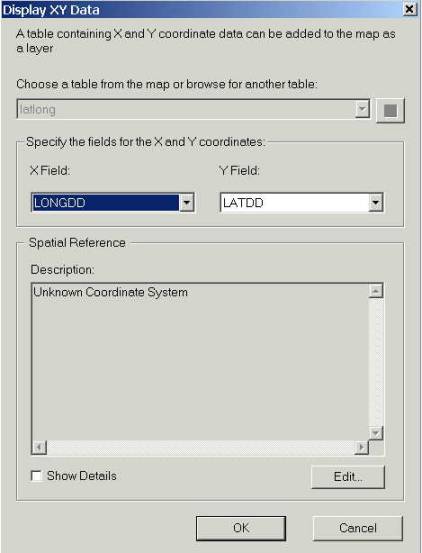
(1) In ArcMap, add the latlong.dbf table created in Excel. Right click on the table and select Display XY Data ..., this will cause a window to appear. The correct x and y fields are selected by ArcMap. Press OK to complete the process of transferring the table to an Event. An event is a point or line that is displayed using coordinates but is not an explict point or line shapefile or feature class. What you’ve done is actually pretty amazing because ArcMap has recognized that the data you created are in geographic coordinates, and it has automatically projected them to the correct coordinate system (an Albers Equal Area Projection) to place them on the map!!! In previous versions of ArcInfo and ArcView, this task was a lot more difficult to carry out.
(2) Create a shapefile out of the XY Event by first right clicking on the latlong Event layer and press Data/Export... to export the data as a shapefile. Name the file albstat.shp and add it to the Map. The gages are on top of the rivers at the right place! This is actually pretty amazing because ArcMap has recognized that the data you created are in geographic coordinates, and it has automatically projected them to the correct coordinate system (an Albers Equal Area Projection) to place them on the map!!!
(3) Save your File and Close ArcMap.
To be turned in: a layout or screen capture of the albstat.shp attribute table with the map.
Add Attributes to the Point Shapefile
Now we are going to add the USGS gage Id, gage name, and annual discharge for each gage as a new attribute in ArcCatalog. (1) Open ArcCatalog and navigate to the folder that contains your data.
(2) Right click on the albstat.shp file and open Properties. Click on the Fields tab and scroll down to the end of the Field Name list. Type the following
|
Field
Name |
Data
Type |
|
USGSID |
Text |
|
Name |
Text |
|
Flow |
Long
Integer |

(3) Click OK and open ArcMap.
Adding Data to the Attribute Table
(1) Right click on the albstat.shp file and open the attribute table. Scroll to the right until you see the new fields you have created. Started editing by selecting Editor/Start Editing.
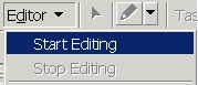
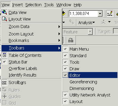
If the Editing Toolbar is not visible it maybe added by selecting View/Toolbars/Editor.
(2) You may now just add the appropriate data values to the table. Continue adding the data values until they are all done.
The following data are needed in the table:
Number USGSID Name Flow 1 08176500 Victoria 20952 08175800 Cuero 2094 3 08168500 New_Braunfels 552 4 08167800 Sattler 464 5 08167000 Comfort 215 6 08166200 Kerrville 1867 08165500 Hunt 81
(3) Select Editor/Stop Editing to finish editing and say Yes when it asks if you would like to save your edits. Note that you can only edit tables for which you have write permission (i.e. your own tables not tables in my work area).
Labeling the Gages in the View
Now you can use the Name field that you've added as a label for the gages.
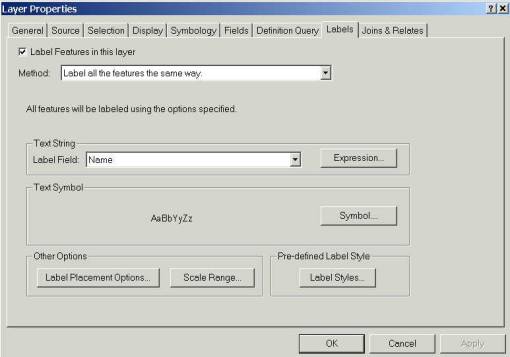
(1) Right Click on the albstat.shp file and select Properties. Click on the Label tab and from the drop down menu select the label field to be Name. Click OK.
(2) Right click on the albstat.shp file again and select Label Features. You can now create a view like this:
Pretty awesome!
Creating a Chart and Layout
(1) Open Excel to create a chart of the mean annual flow of the Guadalupe gages. Open the albstat.dbf file and make a chart using the tools available in Excel. The chart may look something like this

(2) Prepare a layout showing a map of the drainage area, the graph of its annual flows at each gage and a table of numerical values describing the gages. You can import your Excel chart and worksheet from the Insert/Object... option. If necessary resize the original chart or table smaller so that it can be displayed in the layout. You'll see in the chart that the flow in the Guadalupe River at Cuero and Victoria is much higher than in the upstream stations. That is because the flow from the San Marcos river joins the Guadalupe upstream of Cuero.
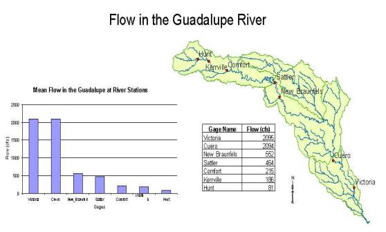
To be turned in: a layout showing the base map, chart and data table for the Guadalupe River flows
Overlaying the Edwards Aquifer
The Edwards aquifer is one of the most critical water resources of Central Texas. It is the main source of water supply for San Antonio, the 10th largest city in the United States. The Edwards aquifer is recharged by infiltration from rivers crossing its outcrop area. To determine where the Guadalupe river crosses, the outcrop area, I obtained a coverage of the Edwards aquifer from the Texas Natural Resource Information System (http://www.tnris.state.tx.us/) by selecting through the menu system: Digital Data, Data Catalog, Water Resources, Ground Water, Major Aquifers where the file Edwards_dd.zip is found. I downloaded this file by logging in to TNRIS using anonymous ftp to: ftp://ftp.tnris.state.tx.us/Water_Resources/Ground_Water/Maj_Aqu_DD/. Use binary in ftp before downloading files from this area. It seems that you should be able to download this from Netscape but the file displayed on the screen when I did this so I used anonymous ftp to get it directly.
The edwards aquifer coverage from TNRIS is in Decimal Degree coordinates. We are using an Albers projection because it preserves earth area. I projected the edwards coverage to Albers TSMS coordinates. This is the Edwards shapefile that you copied from the zip file at the beginning of the exercise.
(1) Add the Edwards shapefile to your ex2 map display.
(2) Click on its Symbology and label the theme using the attribute Aquifer. This attribute has three values: 1 for outcrop, 2 for downdip and 0 for holes within the outer boundary of the aquifer. Classify the values with Unique Value and color them appropriately.
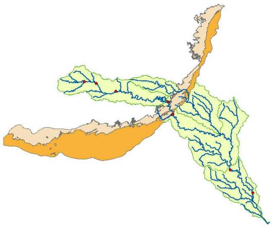
You'll see that the Guadalupe river flows South East towards the Gulf Coast and
it cross first the outcrop and then the downdip portions of the Edwards
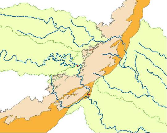
aquifer. The downdip region is where the aquifer dips below the land surface
and is shielded from the surface rivers by overlying hydrogeological units of
low permeability. The Edwards is a fissured limestone aquifer whose fissures
lie along its Southwest to Northeast orientation, so its flow moves in that
direction, transverse to the direction of flow in the Guadalupe basin. It is
thus quite possible for water to drain from the Guadalupe river into the
Edwards aquifer and then reappear as a spring further North in another river,
such as Comal springs feeding the Comal river. (3) Zoom in to the region where
the aquifer crosses the Guadalupe basin for a closer look.
To be turned in: Between which two gaging stations does the Edwards aquifer
outcrop area occur? What is the difference in mean annual flow at these two
gages? Comment on these data. Do they seem correct to you?
Downloading USGS Flow Data
There are also other sources of flow data. One of them is real time data via Internet from the U.S. Geological Survey (http://water.usgs.gov/realtime.html). This data is taken at the site every 15-60 minutes and is transmitted to the USGS office every 1 to 4 hours. This data relayed using satellite, telephone, and/or radio and can be viewed within minutes on arrival to the office.
(1) Click on the site http://water.usgs.gov/realtime.html.
(2) Once you have looked around a bit click on Texas on the map of the United States located above. This link will bring you to a web page,which shows real time data for the state of Texas. Scroll down to the Guadalupe River basin and select the station: Guadalupe Rv at Victoria, TX (08176500).
(3) The new page allows you to change your display options with this toolbar
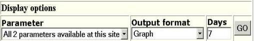
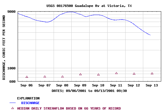
(4) Select your parameter as Discharge, output format as Graph, and Days as 30. Then click on the "Go" button (Retrieving the graph may take awhile). Pretty cool! You can also download tab delineated data from this source so that you create graphs in Excel
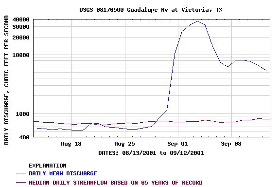
To be turned in: The graph of flow of the Guadalupe River at Victoria printed from the NWIS website and a graph of the discharge from another of the USGS stations on the Guadalupe River. In ArcMap you can copy this graph into a Layout and add a small map to indicate where the data were measured. Or in Excel, you can copy a map into a graph to show where data were measured. What is the current water condition in the Guadalupe Basin? Do something cool!
Ok! You're done!